Welcome back to Writing Math in LaTeX! This is lesson five of seven, which means we are in the home stretch of the course. So far, we have covered math mode, subscripts and superscripts, fractions with \frac, and roots with \sqrt. Each of those tools helped us reproduce the visual structure of mathematical notation. Today we tackle something different — not a new shape or layout, but a naming convention: how to typeset standard function names like $\sin$, $\cos$, $\log$, $\ln$, and $\lim$ so they look the way they should in any published math document.

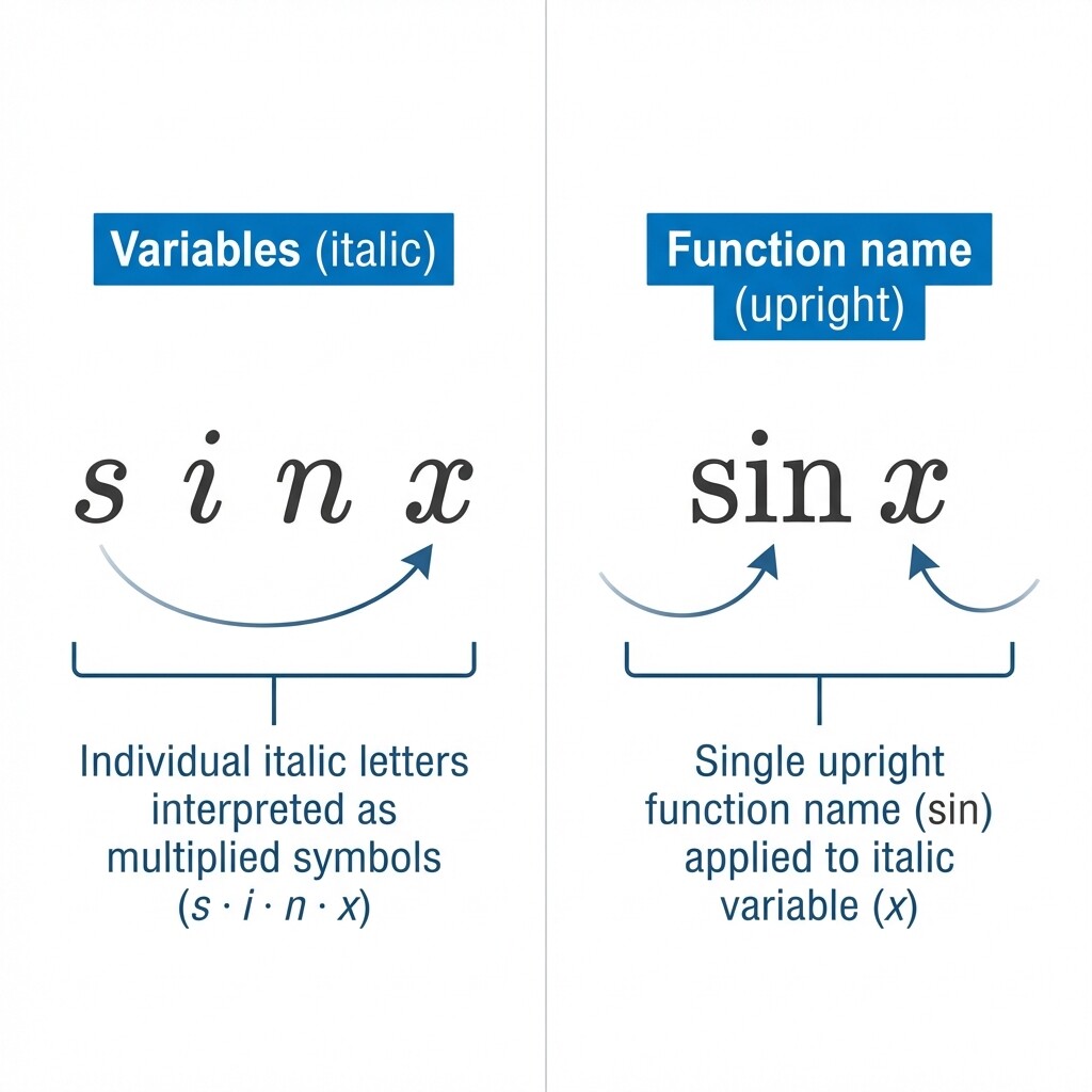
Before we look at any LaTeX commands, it helps to understand a key typographic rule. In mathematics, variables are written in italic type ($x$, $y$, $n$), while function names are written in upright (roman) type ($\sin$, $\log$, $\lim$). This distinction is not just decorative — it tells the reader at a glance whether a group of letters represents a single named function or a product of separate variables.

Let us see what happens when we type the letters sin directly in math mode without any special command:

LaTeX treats each letter as a separate italic variable, producing $s i n x$. This looks like four variables multiplied together — definitely not what we mean. Now compare that with the correct approach:

This produces $\sin x$, where "sin" appears in upright roman type and a small amount of space separates it from $x$. The difference is unmistakable: one reads as a function applied to a variable, the other as a string of multiplied unknowns.

LaTeX provides built-in commands for all the standard mathematical functions you are likely to encounter. Here are the most common ones:

The underscore _ and caret ^ that we learned in Lesson 2 work naturally with function commands. A common example is a logarithm with a specified base:

This produces $\log_2(x)$, where the 2 sits as a subscript to indicate base-2 logarithm. For a base with more than one character, we group with curly braces as usual: $\log_{10}(x)$ gives $\log_{10}(x)$.

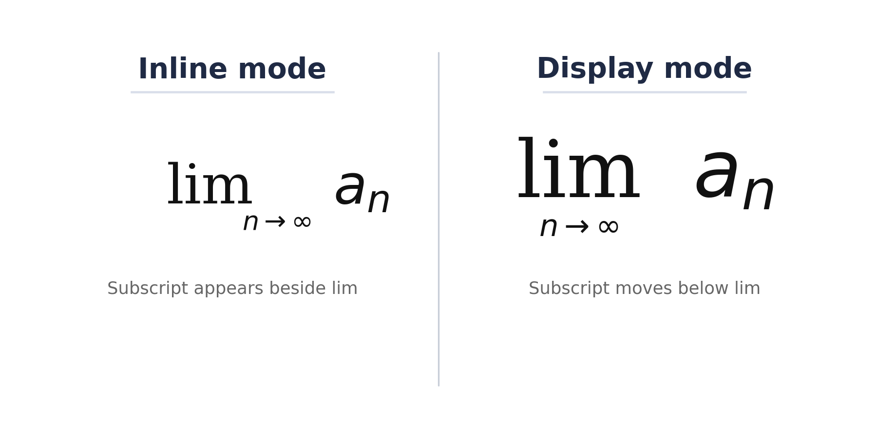
The \lim command deserves a closer look because its subscript behaves differently depending on the math mode.

To write a meaningful limit, we need two more commands that we will preview here: \to produces the arrow $\to$ (read as "approaches"), and \infty produces the infinity symbol $\infty$. Both belong to the broader family of mathematical symbols we will explore in the final lesson of this course, but they show up so often in limits that it makes sense to introduce them now. Consider this expression:

In inline mode, the subscript appears to the side: $\lim_{n \to \infty} a_n$. This keeps the line height compact within a paragraph. But when we switch to display mode:

Now let us combine function commands with the notation we have practiced throughout this course. One of the most famous identities in trigonometry is the Pythagorean identity, which uses \sin, \cos, superscripts, and a Greek letter:

In this lesson, we learned that LaTeX provides dedicated commands like \sin, \cos, \log, \ln, and \lim to typeset standard function names in upright roman type. This keeps function names visually distinct from italic variables — a core convention in mathematical writing. We also saw how these commands combine naturally with subscripts, superscripts, and fractions to build real formulas such as the Pythagorean identity and the change-of-base formula.

Head to the exercises to put these ideas into practice. You will start by comparing raw letters against proper function commands, then build expressions with \log and \lim using subscripts, and finish by assembling a complete trigonometric identity from scratch. In the next lesson, we will explore Greek letters, giving us access to the full alphabet of mathematical symbols.