In the previous three lessons, you built a ray tracer capable of rendering smooth, antialiased images of matte surfaces with realistic lighting. You implemented Lambertian diffuse materials that scatter light randomly in all directions, creating the soft, non-shiny appearance of materials like chalk, unfinished wood, or matte paint. You also fixed two important visual artifacts: shadow acne caused by floating-point precision errors and incorrect brightness perception through gamma correction. Your ray tracer now produces clean, properly lit images with natural-looking diffuse surfaces.

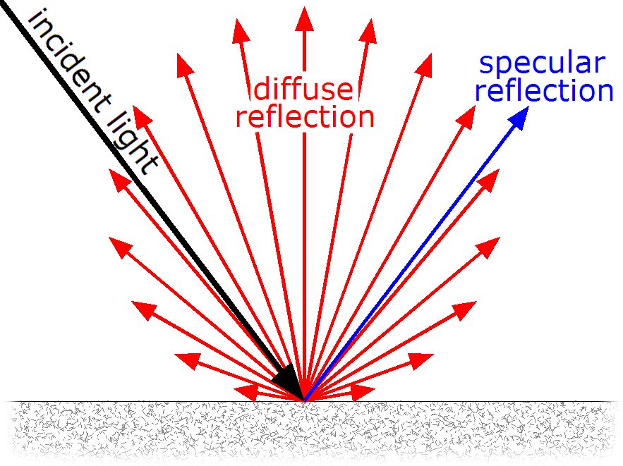
However, if you look around the real world, you'll notice that not everything is matte. Many materials have shiny, reflective surfaces that behave very differently from the diffuse materials we've implemented so far. Think about a polished chrome bumper on a car, a stainless steel refrigerator, a silver spoon, or a brass doorknob. These metallic surfaces don't scatter light randomly like matte materials do. Instead, they reflect light in a mirror-like way, bouncing incoming rays in a specific direction determined by the surface angle. When you look at a polished metal surface, you can often see reflections of other objects in the scene, and the surface itself appears bright and shiny rather than soft and matte.

In this lesson, you'll learn how to add metallic materials to your ray tracer by implementing reflection. You'll understand the mathematics behind reflection vectors and how they differ from the random scattering we used for diffuse materials. We'll start by implementing perfect mirror-like reflection, which simulates highly polished metals like chrome or polished silver. Then we'll extend this to handle fuzzy or rough reflection, which models metals with slightly imperfect surfaces like brushed aluminum or worn steel. By the end of this lesson, you'll be able to render scenes containing both matte and shiny surfaces, with metals that reflect their surroundings and add visual interest to your images.

The key difference between diffuse and metallic materials lies in how they handle incoming light rays. As you learned in Lesson 2, diffuse materials scatter light randomly in all directions according to the Lambertian model. When a ray hits a diffuse surface, the scattered ray direction is chosen randomly from a hemisphere around the surface normal, with no relationship to the incoming ray direction. Metallic materials, on the other hand, follow the law of reflection: the outgoing ray direction is determined precisely by the incoming ray direction and the surface normal. This predictable, mirror-like behavior is what gives metals their characteristic shiny appearance and their ability to reflect clear images of their surroundings.

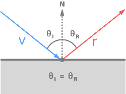
The foundation of rendering metallic surfaces is understanding how light reflects off smooth surfaces. The behavior of reflection is governed by a fundamental principle in optics called the law of reflection, which states that when a light ray strikes a reflective surface, the angle at which it arrives (the angle of incidence) equals the angle at which it departs (the angle of reflection). Both of these angles are measured relative to the surface normal, which is the line perpendicular to the surface at the point where the ray hits.

To visualize this, imagine a ball bouncing off a flat floor. If you throw the ball straight down, it bounces straight back up. If you throw it at an angle, it bounces off at the same angle on the other side. The floor's normal is the vertical line pointing straight up from the floor, and the ball's incoming and outgoing paths make equal angles with this vertical line. Light behaves the same way when it reflects off a smooth surface. The incoming ray, the surface normal, and the reflected ray all lie in the same plane, and the angles on either side of the normal are equal.

Mathematically, we can calculate the reflected ray direction using a formula that takes the incoming ray direction and the surface normal as inputs. If we call the incoming ray direction vector v and the surface normal n, the reflected direction r is given by the formula r = v - 2(v · n)n. The dot product (v · n) measures how much the incoming ray is pointing toward or away from the normal. Multiplying this by the normal and then by two gives us a vector that, when subtracted from the original direction, produces the reflection.

To understand why this formula works, think about what we're trying to do geometrically. We want to flip the incoming ray direction across the normal, like folding a piece of paper along a crease. The component of the incoming ray that's parallel to the surface stays the same, but the component perpendicular to the surface (pointing into or out of the surface) needs to be reversed. The term 2(v · n)n represents twice the perpendicular component of the incoming ray. When we subtract this from the original ray direction, we're effectively removing the perpendicular component and adding it back in the opposite direction, which gives us the reflection.

Now that we understand the mathematics of reflection, let's implement it in code. We'll add some mathematical utility functions like reflection to our header file called math_utils.h. As your ray tracer grows, you'll likely add more mathematical operations to this file, such as refraction for glass materials or other vector operations. Keeping these utilities separate from the main rendering code helps keep your project organized and makes the functions easy to reuse.

Add to the file src/math_utils.h the following content:

This is a straightforward implementation of the reflection formula we discussed. The function takes two parameters: the incoming ray direction v and the surface normal n. Both are passed by constant reference to avoid unnecessary copying. The function returns a new vec3 representing the reflected direction. The calculation follows the formula exactly: we compute the dot product of the incoming direction and the normal, multiply by two and by the normal vector, and subtract this from the incoming direction.

The inline keyword suggests to the compiler that it should try to insert the function's code directly at each call site rather than making a function call. For small, frequently called functions like this, inlining can improve performance by eliminating the overhead of function calls. Modern compilers are quite good at deciding when to inline functions, so this keyword is more of a hint than a command, but it's good practice for small utility functions.

With our reflection function implemented, we're ready to create a new material type for metallic surfaces. As you'll recall from Lesson 2, we have a material system based on an abstract material class with a virtual scatter function. The lambertian class implements diffuse scattering by generating random directions. Now we'll add a metal class that implements specular reflection using our new reflect function.

Open src/material.h and add the new metal class after the lambertian class. First, make sure to include our new math utilities header at the top of the file:

Now add the metal class definition:

Let's start by understanding the simpler case of perfect reflection before we discuss the fuzz parameter. The constructor takes an albedo color and a fuzz value. The albedo represents the color tint of the metal. Real metals aren't perfectly white reflectors. Gold has a yellowish tint, copper is reddish, and even silver has a slight bluish tint. The albedo lets us simulate these colored metals by tinting the reflected light. We store the albedo as a member variable so we can use it in the scatter function.

Perfect mirror-like reflection looks great for highly polished metals like chrome or a freshly polished silver mirror. However, most real-world metals aren't perfect mirrors. If you look at a stainless steel refrigerator, brushed aluminum laptop case, or a slightly worn brass doorknob, you'll notice that while they're still shiny and reflective, the reflections are somewhat blurred or fuzzy. You can see the general shapes and colors of reflected objects, but the details aren't as sharp as in a perfect mirror. This happens because real metal surfaces have microscopic imperfections and roughness that scatter the reflected light slightly.

At a microscopic level, even a seemingly smooth metal surface has tiny bumps, scratches, and irregularities. Each of these microscopic features acts like a tiny mirror with its own normal direction. When light hits the surface, different parts of the incoming beam reflect off these tiny facets in slightly different directions. The overall effect is that the reflected light spreads out into a small cone around the perfect reflection direction rather than reflecting in a single precise direction. The rougher the surface, the wider this cone of reflected light becomes.

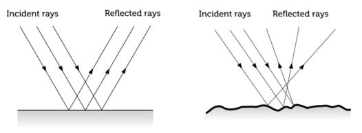
We can simulate this effect in our ray tracer by adding a small random perturbation to the perfect reflection direction. Instead of scattering the ray exactly along the calculated reflection vector, we add a random offset that pushes the ray slightly away from the perfect reflection. The amount of this offset is controlled by a parameter we call the fuzz factor. A fuzz of zero means no perturbation, giving us perfect mirror-like reflection. A larger fuzz value means more perturbation, creating a rougher, more diffuse reflection that looks like brushed or worn metal.

The fuzz parameter typically ranges from zero to one. At fuzz equals zero, we get perfect specular reflection like a polished mirror. As fuzz increases toward one, the reflection becomes increasingly scattered and blurry. At fuzz equals one, the reflection is so scattered that the material starts to look almost diffuse, though it's still fundamentally different from a Lambertian material because the scattering is centered around the reflection direction rather than the surface normal. Values greater than one would create unrealistic behavior where the scattered rays spread too widely, so we clamp the fuzz parameter to a maximum of one.

Think of fuzz as representing the microscopic roughness of the surface. A highly polished chrome bumper might have a fuzz of 0.0 or 0.05, giving nearly perfect reflections. Brushed stainless steel might have a fuzz of 0.3, creating noticeably softer reflections. A very rough, oxidized metal surface might have a fuzz of 0.7 or higher, where reflections are quite blurred and the surface looks less mirror-like. This single parameter gives us a wide range of metallic appearances, from perfect mirrors to rough, worn metals.

Looking back at the metal class code we showed earlier, you can now understand the complete implementation including the fuzz parameter. The constructor takes both an albedo color and a fuzz value. We clamp the fuzz value to a maximum of one using a conditional expression: fuzz(f < 1 ? f : 1). This ensures that even if someone passes a fuzz value greater than one, we'll use one instead, preventing unrealistic behavior.

In the scatter function, after calculating the perfect reflection direction, we generate the fuzz perturbation:

The random_unit_vector() function returns a random direction on the unit sphere, just as we used for diffuse materials. Multiplying by the fuzz factor scales this random vector. If fuzz is zero, fuzz_dir becomes the zero vector and we get perfect reflection. If fuzz is 0.3, the random vector is scaled to thirty percent of its original length, creating a small perturbation. If fuzz is one, we use the full random vector, creating maximum scattering while still being centered around the reflection direction.

Adding this fuzz direction to the perfect reflection direction gives us the final scattered ray direction. This is vector addition, so we're offsetting the reflection direction by a random amount. The scattered ray still generally points in the reflection direction, but it's been nudged randomly. The larger the fuzz, the larger the possible nudge, and the more scattered the reflections become.

The final check return (dot(scattered.direction(), rec.normal) > 0) becomes especially important with fuzzy reflection. When we add a random perturbation to the reflection direction, there's a chance the perturbed direction might point below the surface, especially for large fuzz values or for rays hitting the surface at grazing angles. If the dot product of the scattered direction and the normal is negative or zero, the scattered ray would be going into or along the surface, which is physically impossible. In this case, we return false, telling the ray tracer to absorb the ray rather than scatter it. This absorption is the correct physical behavior and prevents artifacts from invalid ray directions.

In this lesson, you learned how to add metallic surfaces to your ray tracer by implementing reflection. You explored the law of reflection and the reflection formula v - 2(v · n)n, then encapsulated this in a reusable reflect() function. You created a metal material class that uses this function to produce mirror-like reflections, with the albedo parameter controlling the color tint of the metal. To simulate real-world surface roughness, you added a fuzz parameter that perturbs the reflection direction, allowing you to render everything from perfect mirrors to rough, brushed metals. You also learned the importance of ensuring scattered rays point away from the surface. With both diffuse and metallic materials, your ray tracer can now render a wide variety of realistic surfaces. In the next practices, you’ll experiment with different metal configurations and fuzz values to see their effects, preparing for even more advanced materials like glass in future lessons.