Stabilization Over Trials
Introduction
Have you ever noticed that a single data point can mislead you completely, while a long series of observations tends to tell a much steadier story? That shift — from noisy early estimates to a calm, reliable value — is exactly what this lesson is about. With three of four lessons now underway, you are three-quarters of the way through this course.
In Lesson 1, you learned to compute relative frequency as a data-driven estimate of true probability. In Lesson 2, you saw why small samples make that estimate fragile: when is tiny, a single observation can swing the ratio dramatically. We left off with the natural remedy — collect more data. Today, we examine exactly how more data calms those fluctuations, and what that eventual steady value actually represents.
The Core Intuition
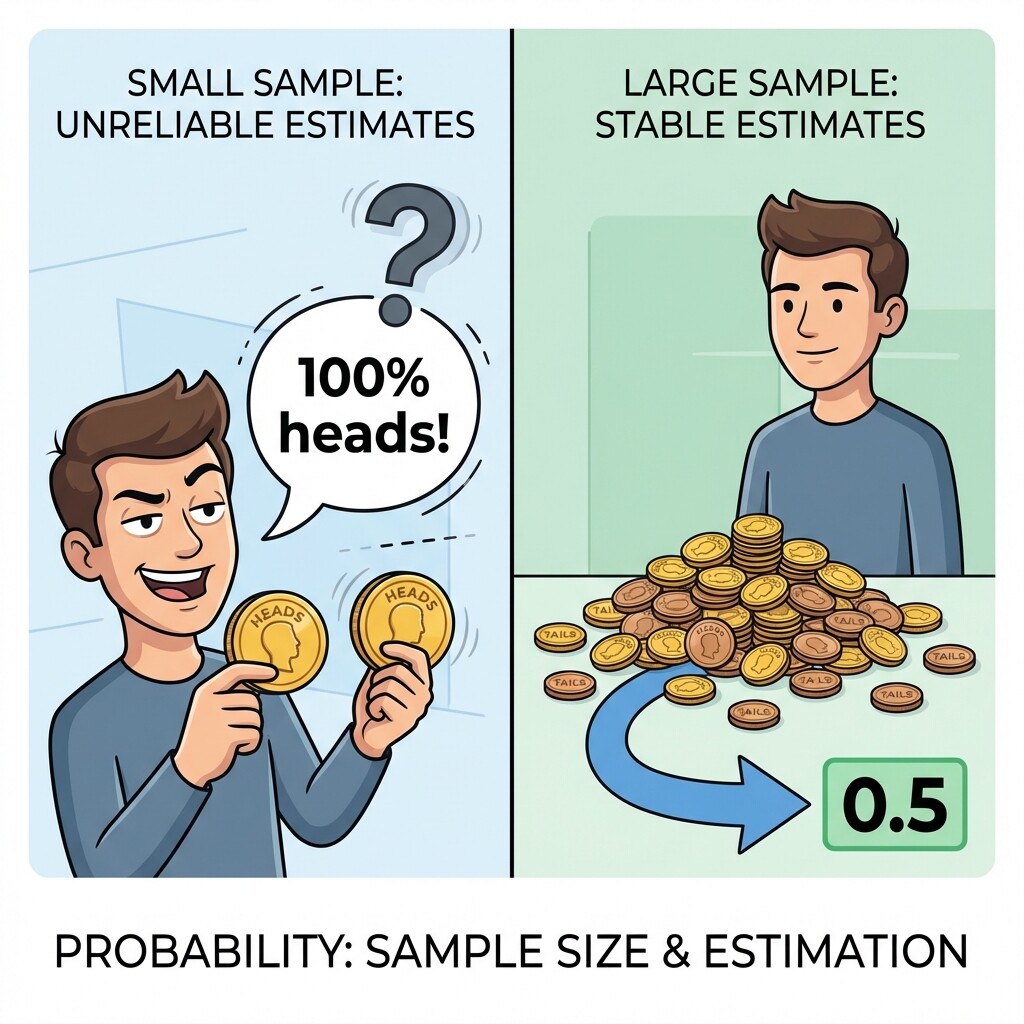
Think about what happens when a friend flips a coin just twice and gets heads both times. They announce that heads comes up 100% of the time. Most of us would immediately push back, sensing that two flips are not nearly enough to reveal anything trustworthy about the coin.
That instinct is correct, and it points to something important: we expect that more repetitions of an experiment will eventually produce a stable, believable estimate. The relative frequency stops jumping around and begins to hover near a particular value. This lesson is about understanding why that happens and what it means.
Running Relative Frequency
To study stabilization closely, we track the relative frequency after every single trial, not just at the end of the experiment. We call this the running relative frequency. The formula is the same one we learned in Lesson 1:
Here, is the total count of times the event has occurred through trial . We simply update this ratio with each new observation.
Consider flipping a fair coin and recording whether each flip lands on heads. The table below shows the running relative frequency for the first 10 trials.
| Trial | Result | Total Heads | Running RF |
|---|---|---|---|
| 1 | Heads | 1 | |
| 2 | Tails | 1 | |
| 3 | Tails | 1 | |
| 4 | Heads | 2 | |
| 5 | Heads | 3 | |
| 6 | Tails | 3 | |
| 7 | Heads | 4 | |
| 8 | Tails | 4 | |
| 9 | Tails | 4 | |
| 10 | Heads | 5 |
The running relative frequency swings noticeably in the early trials. From trial 1 to trial 2 alone, it drops from to — a shift of — just because of a single tails result.
Why Each New Trial Has Less Impact
Here is the key insight. When is small, adding one more trial changes the denominator by a large proportion of the whole. As grows, that same change of becomes a smaller and smaller fraction of the total, so its power to shift the running relative frequency shrinks.
More precisely, the maximum possible change the running relative frequency can experience when moving from trials to trials is:
Let's see how that plays out across a few values of :
| Trials so far | Max shift after one more trial |
|---|---|
| 4 | |
| 9 | |
| 24 | |
| 99 | |
| 499 |
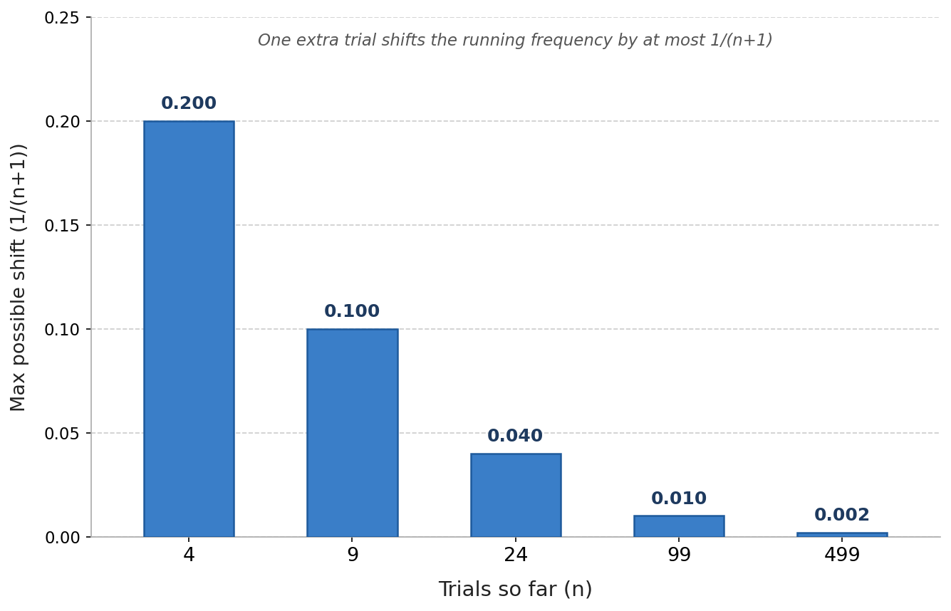
Each successive trial is less able to move the estimate than the one before it. This is exactly why large samples produce stable estimates: the running relative frequency becomes increasingly resistant to the pull of any single new result.
Watching It Stabilize
Let's continue our coin-flip example, this time skipping ahead to larger trial counts to see the stabilization effect in action.
| Trials so far | Total Heads | Running RF |
|---|---|---|
| 10 | 5 | |
| 25 | 11 | |
| 50 | 23 | |
| 100 | 48 | |
| 200 | 99 | |
| 500 | 251 |
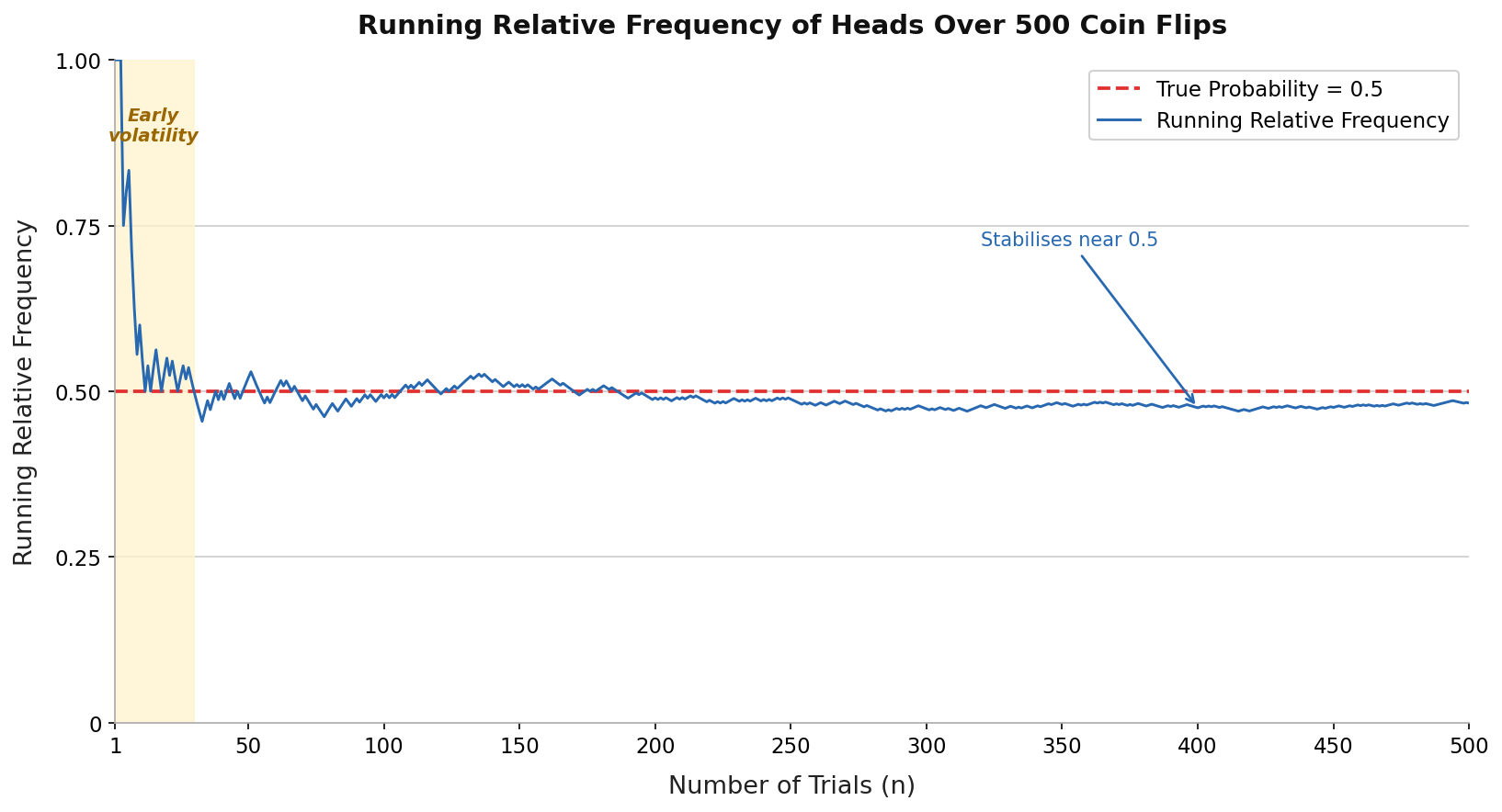
The running relative frequency still moves, but notice how much smaller those movements become. Early on, values like and appeared within just a few trials. By trial 500, the estimate barely budges from one checkpoint to the next. If we plotted this on a graph, we would see a jagged line at the start that gradually flattens out near a particular value. That flattening is the visual signature of stabilization, and we will explore it hands-on in the practice exercises.
Connecting Stabilization to True Probability
The value the running relative frequency settles near is not random — it is tied directly to the underlying process. For our fair coin, it settles near because that is the true probability of heads. For a coin weighted so that heads comes up 30% of the time, the running relative frequency would drift toward instead. The same idea applies in many real-world settings: a quality inspector checking thousands of manufactured parts will find the proportion of defective items converging on the true defect rate, and a meteorologist tracking daily weather over many years will see the relative frequency of rainy days approach the city's genuine long-run probability of rain.
The general principle is:
As the number of trials grows large, the relative frequency tends to approach the true probability of the event.
This idea is known informally as the Law of Large Numbers. We do not need its formal mathematical proof here. What matters is the practical takeaway: running enough trials gives us an experimental estimate that can reliably stand in for a true probability we may not be able to calculate directly.
One important clarification: stabilization does not mean the running relative frequency ever becomes perfectly equal to the true probability. Small random deviations always persist. What changes is that those deviations shrink in size, and the estimate stays within an increasingly narrow band around the true value.
Conclusion and Next Steps
In this lesson, we traced how the running relative frequency of an event evolves as trials accumulate. Early estimates fluctuate widely because each observation carries a large share of the ratio, but as grows, the maximum possible shift shrinks with every trial, and the estimate settles near the event's true probability — a principle known as the Law of Large Numbers.
Now it is time to see this come alive. The upcoming practice will have you watching stabilization unfold in real time through an interactive simulation, reading graphs for its visual signature, and expressing the pattern in your own words — the kind of hands-on experience that transforms an idea you understand into one you truly own.
