Over the past three lessons, we built up a complete picture: computing relative frequency as a data-driven estimate, understanding why small samples produce unstable results, and watching how those estimates gradually settle near the true probability as more data accumulates. Now it is time to bring all of those ideas together into one clear, practical skill: estimating probability from real data and evaluating how much that estimate can be trusted.
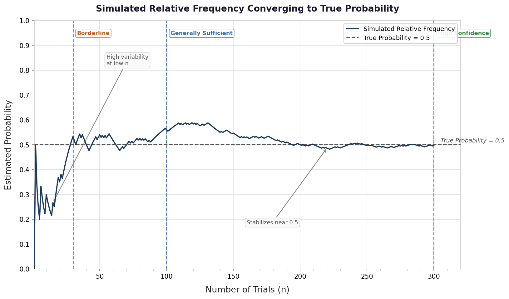
As you may recall from Lesson 3, the relative frequency of an event tends to stabilize near its true probability as the number of trials grows — a principle known as the Law of Large Numbers. That stabilization is precisely what makes experimental estimation useful: once enough data has been collected, the relative frequency becomes a reliable stand-in for a true probability we might not be able to calculate directly.
This matters especially in real-world situations where the true probability cannot be determined by logic alone. Suppose you want to know the probability that a customer will leave a positive review, or that a particular flight will arrive on time. These events have no clean, theoretical answers — but with enough observed data, you can build a solid estimate from what actually happened. The recorded outcomes become your evidence.
This final lesson focuses on two connected questions. First, how do we produce a probability estimate from a real data set? Second, how do we decide whether we have collected enough data to trust that estimate? By the end, you will have a clear, repeatable process for answering both.
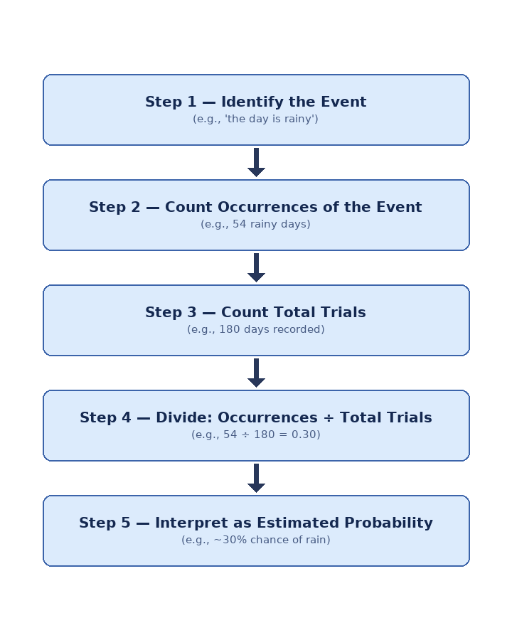
The estimation procedure uses the same relative frequency formula introduced in Lesson 1. Given a data set, we apply:
The symbol means "approximately equal to," which is appropriate because any estimate derived from experimental data is, by nature, an approximation.
A probability estimate is only as good as the data behind it. As we saw in Lesson 2, small samples can produce estimates that shift dramatically with just one or two additional observations. Before reporting an estimate, it is worth asking: do we have enough trials for this result to be reasonably stable?
There is no single universal cutoff, so it is better to think of sample size as a continuum rather than a set of sharp categories. A rough guide is:
These are only rough guidelines, not hard rules: a sample of 99 is not fundamentally different from a sample of 100. The underlying principle is the one from Lesson 3: as the number of trials grows, the maximum possible shift caused by any single new observation, , shrinks. A larger sample means the estimate has had more chances to settle near the true probability, and each additional result carries less power to disturb it.
In real-world situations, you may come across two different probability estimates for the same event, each based on data sets that vary greatly in size. Generally, the estimate from the larger sample tends to be more reliable.
That said, sample size alone isn't everything — the way a sample is constructed matters just as much.
For example, imagine you want to estimate how many people in a city prefer public transport over driving. Sample A surveys 10,000 people, but all of them were interviewed at a subway station during rush hour. Sample B surveys only 500 people, but they were randomly selected from across the entire city. Despite being far smaller, Sample B is likely to produce a more accurate estimate, because Sample A is heavily skewed toward people who already use public transport. A large but biased sample can be more misleading than a small but representative one.
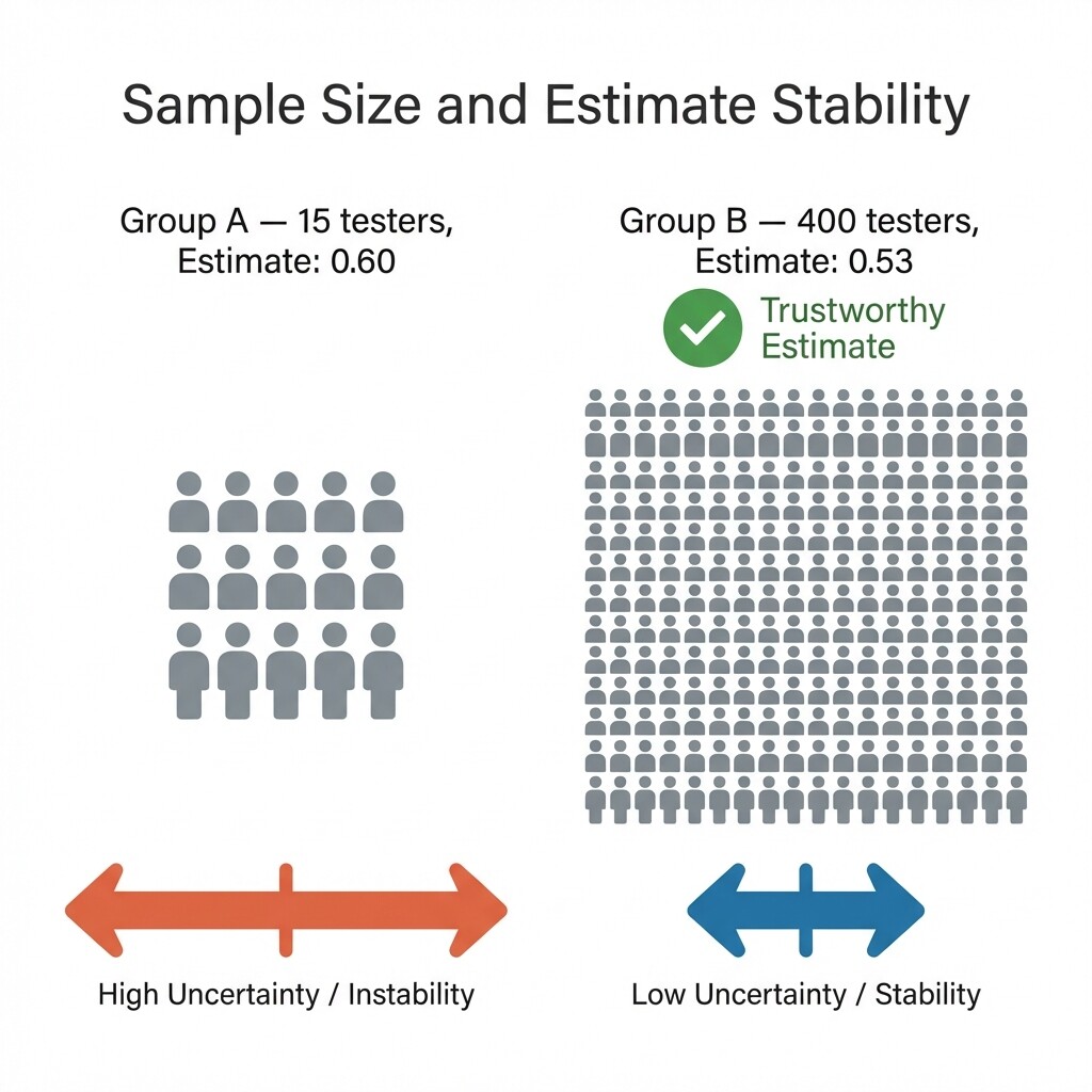
However, if two samples have a similar structure and are equally representative, you should trust the bigger one. Consider this scenario: a software company tests a new feature with two groups of randomly selected users. Group A has 15 testers; 9 of them found the feature useful, giving an estimate of . Group B has 400 testers; 212 found the feature useful, giving an estimate of . Both suggest that a majority of users find the feature useful, but which estimate is more trustworthy?
In this final lesson of Probability from Experiments, we brought together the skills from all three previous lessons into a complete estimation workflow. We applied the relative frequency formula to a real data set, evaluated whether a sample is large enough to support a trustworthy estimate, and compared two estimates to identify the one backed by stronger evidence.
The practice section ahead will take you through realistic data sets — from customer feedback to travel records — where you will compute estimates, judge their reliability, and express your reasoning in your own words. That hands-on variety is exactly what transforms a concept from something understood into something truly mastered.