Welcome! Today's focus is on t-SNE parameter tuning using R and the Rtsne package. This lesson covers an understanding of critical t-SNE parameters, the practice of parameter tuning, and its impact on data visualization outcomes in R.

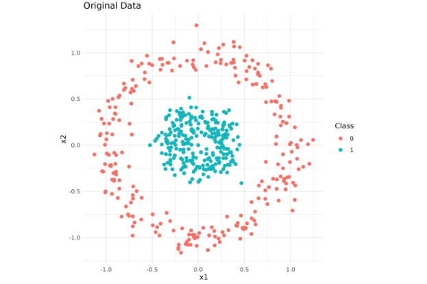
Before delving into parameter tuning, let's quickly set up the dataset:

Here's a basic setup in R:

We will now delve into the key parameters in R's t-SNE implementation (Rtsne). The first one is perplexity, which is loosely determined by the number of effective nearest neighbors. It strikes a balance between preserving the local and global data structure.

The next parameter is exaggeration_factor (in Rtsne, this replaces early_exaggeration). It governs how tight natural clusters are in the embedded space. High values tend to make clusters denser.

The final parameter, eta, modulates the step size for the gradient during the optimization process.

Now that our dataset is prepared, we have the freedom to adjust the t-SNE parameters and observe the visual impact.

We can compare the results of t-SNE with default parameters and custom ones side by side using facets in ggplot2.

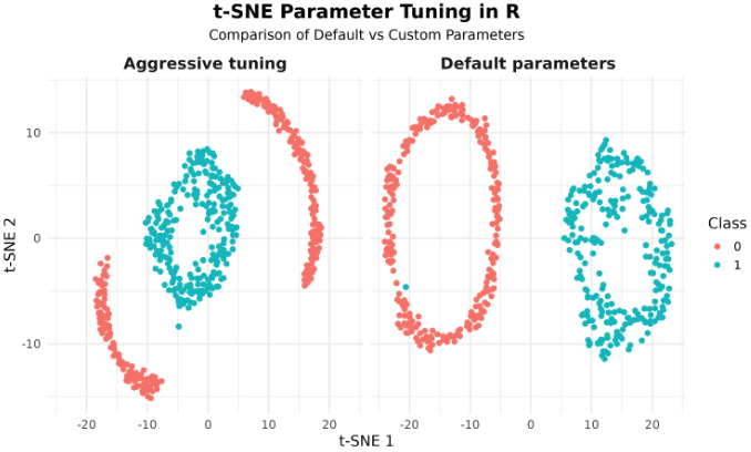
Note: Results can differ slightly due to randomness in initialization and implementation details. If you prefer the original mlbench.circle, expect less separation (smaller radial gap). The above generator mirrors make_circles(factor=0.3, noise=0.1) to make the effect of parameter tuning more visible.

In conclusion, mastering t-SNE in R using the Rtsne package involves understanding and effectively adjusting its tunable parameters. Throughout this lesson, we've explored parameter tuning in Rtsne, understood the impact of key parameters, and experimented with different parameter settings. Now, gear up for hands-on practice to couple theory with application. It's time to practice and excel in t-SNE!