Welcome to the fascinating world of Locally Linear Embedding (LLE), a vital tool in our dimensionality reduction toolbox. Unlike linear techniques like Principal Component Analysis (PCA), LLE shines at preserving local neighborhood structure in high-dimensional data.
In this lesson, we’ll unpack the LLE algorithm, discuss when to use it, and contrast it with PCA. We’ll implement it in R, using ggplot2 for visualization and a small helper we’ll write to run LLE.
LLE preserves relationships within local neighborhoods while reducing dimensionality, capturing twists and turns in non-linear manifolds (e.g., images, pose, genomics). Like reading a street map vs. a bird’s-eye projection: PCA may distort local distances, whereas LLE maintains them.
We’ll use the Swiss Roll—a classic 3D manifold that’s hard for linear methods but perfect for LLE.
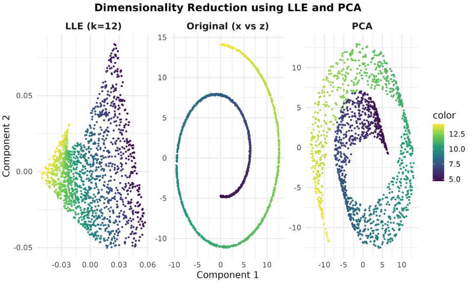
We’ll compare the original Swiss Roll projection (x vs z) with LLE and PCA in 2D.
You should see LLE unfold the roll into a smooth 2D strip, while PCA tends to smear/overlap the manifold because it’s linear. Look at example below:
We can compute the LLE reconstruction error directly from the weights (same objective as Step 1) and the PCA reconstruction error as the fraction of variance not explained by the first two PCs.
(Exact values vary with noise and sample size, but LLE should be very low; PCA typically leaves notable error on Swiss Roll.)
Congratulations! You’ve explored Locally Linear Embedding (LLE) and contrasted it with PCA using the Swiss Roll dataset. You saw how LLE preserves local neighborhood structure and effectively unfolds a non-linear manifold into 2D, while PCA—being linear—cannot capture these curved relationships.
