Welcome, learners! Today, we embark on an exciting chapter on non-linear dimensionality reduction techniques, focusing on Kernel Principal Component Analysis (Kernel PCA), an extension of Principal Component Analysis (PCA). Kernel PCA enhances the capabilities of PCA by enabling it to handle non-linear relationships in data.

In this lesson, you will learn the theoretical foundations of Kernel PCA, the importance of kernel selection, and how to apply Kernel PCA in practice using R. We will use the kernlab package for Kernel PCA and ggplot2 for data visualization.

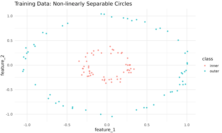
Kernel PCA is a powerful variant of PCA that efficiently handles non-linear transformations through kernel methods. The "Kernel Trick" allows us to map input data into a higher-dimensional feature space, making it possible to separate data that is not linearly separable in the original space.

Kernels are essential for measuring similarity between observations. Choosing the right kernel — such as linear, polynomial, or radial basis function (RBF) — is crucial for the performance of Kernel PCA.

To demonstrate Kernel PCA, we will generate a two-circle dataset (similar to Python’s make_circles). We’ll then split the data into training and testing sets and visualize it using ggplot2.

The plot above shows the two classes forming concentric circles that are not linearly separable.

Now, let's apply Kernel PCA using the kernlab package. We’ll standardize the features first, because RBF kernels are sensitive to scale.

We’ll visualize the eigenvalues of the kernel principal components and the projection of the test data.

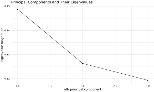
If your projection looks like a line, it means almost all variance is in the first PC. Try changing the sigma_value (or even plotting PC1 vs PC3 if eigenvalue 3 > eigenvalue 2).

We typically evaluate the effectiveness of the transformation by examining the variance captured by each principal component (using the eigenvalues).

This plot helps you decide how many kernel principal components to retain for downstream tasks.

Note: In kernel PCA, the eigenvalues of the kernel matrix provide only an approximate indication of the variance explained by each principal component. Unlike standard PCA, these eigenvalues do not correspond exactly to the variance explained in the original input space, especially if the kernel matrix is not properly centered or normalized. Therefore, use the proportions as a rough guide rather than an exact measure of explained variance.

The kernlab::kpca function offers several hyperparameters:

• kernel: "vanilladot" (linear), "polydot" (polynomial), "rbfdot" (RBF), "tanhdot" (sigmoid), etc.
• kpar: kernel parameters. For "rbfdot", sigma controls the kernel width.
• features: number of principal components to compute.
• th: threshold for variance explained.

Tuning these parameters can help avoid collapsed projections (just a line) and reveal meaningful structure.

Congratulations on completing the lesson on Kernel PCA! You have learned how to generate non-linearly separable data, apply kernel methods, visualize projections, and evaluate the variance explained by kernel principal components in R.

Now experiment with different sigma values and kernels — sometimes the difference between a collapsed line and a rich unfolding is just the right kernel parameter.