Embark on an exciting journey through the world of Principal Component Analysis (PCA). In this lesson, we will explore the indispensable roles of eigenvalues and eigenvectors in understanding the PCA framework and dive into the computation of these mathematical constructs using R. Our adventure will cover the essential role of the covariance matrix and how to compute it. Ready? Set? Let's start!

At the onset, we start with a dataset housing different physical measures: weight_lbs (in lbs), height_inches (in inches), and height_cm (in cm). We capture these in R using vectors and combine them into a data frame for easy manipulation:

# Given data
weight_lbs <- c(150, 160, 155, 165, 170, 160, 158, 175, 180, 170)
height_inches <- c(68, 72, 66, 69, 71, 65, 67, 70, 73, 68)
height_cm <- c(172.72, 182.88, 167.64, 175.26, 180.34, 165.1, 170.18, 177.8, 185.42, 172.72)

# Create a data frame
df <- data.frame(
  weight_lbs = weight_lbs,
  height_inches = height_inches,
  height_cm = height_cm
)

Here, the data frame df represents our collected dataset.

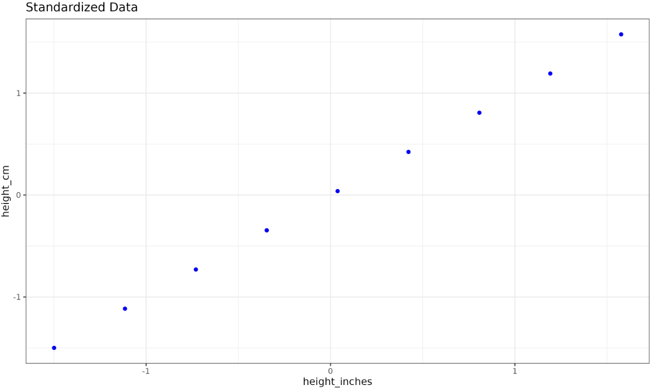
Let's standardize just the two height columns in our dataset using R's scale() function and visualize the standardized data using ggplot2:

library(ggplot2)

# Select the height columns and standardize
X <- df[, c("height_inches", "height_cm")]
X_standard <- scale(X)

# Convert to data frame for plotting
X_standard_df <- as.data.frame(X_standard)
colnames(X_standard_df) <- c("height_inches", "height_cm")

# Plot standardized data
ggplot(X_standard_df, aes(x = height_inches, y = height_cm)) +
  geom_point(color = "blue") +
  ggtitle("Standardized Data") +
  xlab("height_inches") +
  ylab("height_cm") +
  theme_bw() +
  theme(panel.grid = element_line())

Output:

After standardization, our data is now centered and scaled, making the variables more comparable.

Before calculating the covariance matrix, let's understand what it signifies and why it's important in PCA.

Covariance gives us a measure of the extent to which corresponding deviations from averages tend to move together. In other words, it implies how one variable changes in relation to another. Covariance between two variables can be positive, implying the variables increase or decrease together, or negative, meaning one variable increases when the other decreases.

By helping identify the direction with the most variance in data, the covariance matrix lays the foundation for PCA. The eigenvectors, derived from the covariance matrix, will form the new axes along which our data will lie. The corresponding eigenvalues denote the variances along these new axes.

We compute the covariance in R using the cov() function.

# Compute the covariance matrix
cov_matrix <- cov(X_standard)

cat("Covariance Matrix:\n")
print(cov_matrix)

The covariance matrix, cov_matrix, saves the covariance between pairs of features in our scaled dataset. You will see output similar to:

              height_inches height_cm
height_inches      1.111111  1.111111
height_cm          1.111111  1.111111

The covariance matrix is symmetric, with the diagonal elements representing the variance of each feature and the off-diagonal elements representing the covariance between features.

We can understand the following from the covariance matrix:

• Both variables have a variance of approximately 1.11. This indicates similar spread in both variables, which is expected since we standardized them.
• The covariance between the two variables is also about 1.11. This suggests a positive relationship between the two variables, meaning they tend to increase or decrease together.

Let's introduce eigendecomposition into our process. This technique decomposes matrices into their constituent parts and aids in understanding and simplifying complex matrix operations, which is crucial in PCA.

Here, we calculate the eigenvalues and eigenvectors of the covariance matrix using R's eigen() function.

# Eigendecomposition
eig <- eigen(cov_matrix)
eigenvalues <- eig$values
eigenvectors <- eig$vectors

cat("\nEigenvalues:\n")
print(eigenvalues)

cat("\nEigenvectors:\n")
print(eigenvectors)

The eigen() function returns eigenvalues and their corresponding eigenvectors, which help decipher the PCA's underlying structure.

Let's interpret the output (your values may be slightly different due to floating-point precision):

Eigenvalues:
[1] 2.222222e+00 1.110223e-16

Eigenvectors:
           [,1]       [,2]
[1,] 0.7071068 -0.7071068
[2,] 0.7071068  0.7071068

The eigenvalues signify the variance captured by each eigenvector. The first eigenvalue (about 2.22) is significantly higher than the second (very close to zero), indicating the first eigenvector captures most of the variance in the data.

The eigenvectors represent the directions of maximum variance in the data. The first eigenvector [0.7071068, 0.7071068] captures the direction of maximum variance, while the second eigenvector [-0.7071068, 0.7071068] captures the direction of the second highest variance.

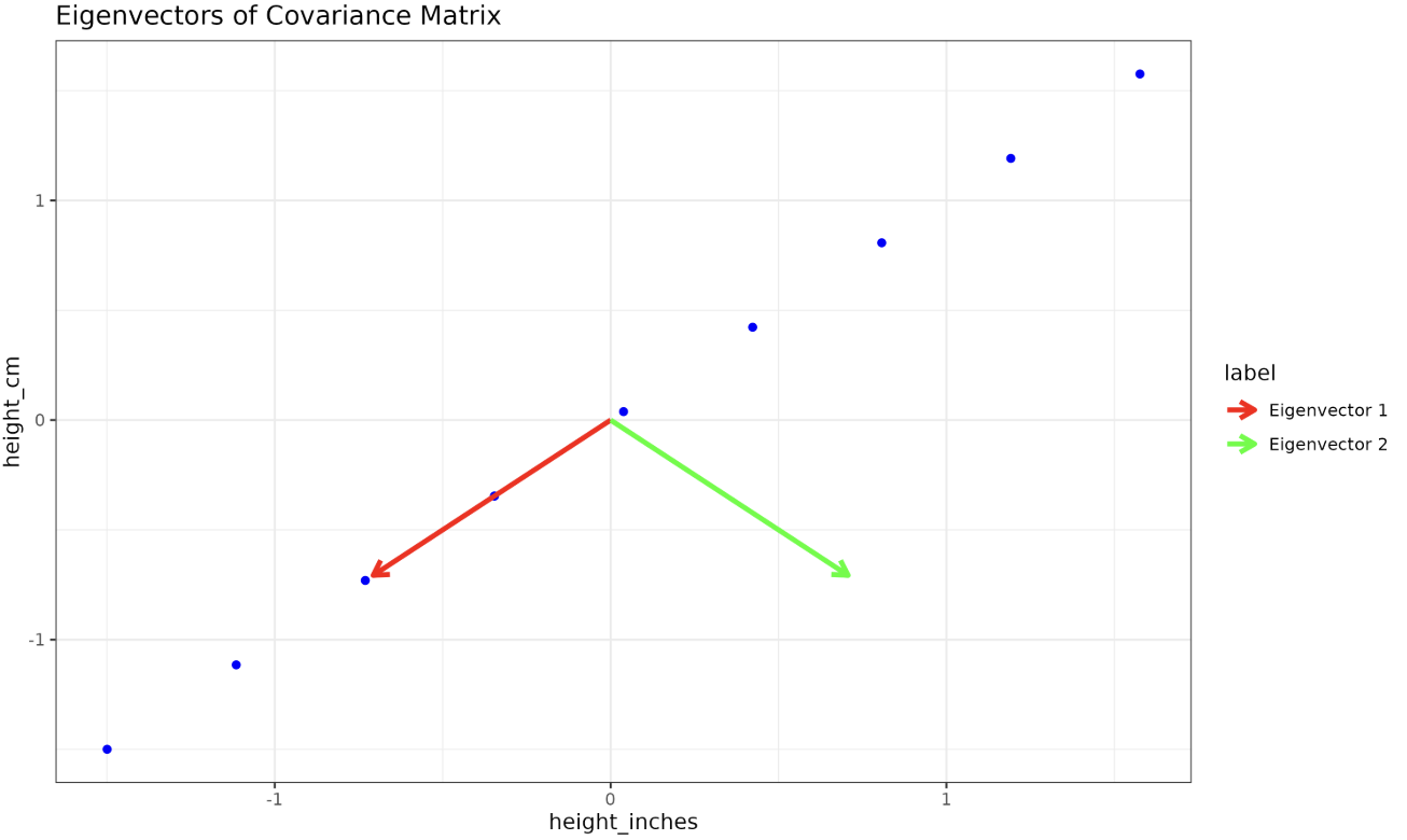
We can plot eigenvectors on a graph to visualize their direction and magnitude. Let's plot the eigenvectors of the covariance matrix we calculated earlier.

library(ggplot2)

# Prepare data for plotting
origin <- data.frame(x = 0, y = 0)
eigvec_df <- data.frame(
  xend = eigenvectors[1, ],
  yend = eigenvectors[2, ],
  label = c("Eigenvector 1", "Eigenvector 2"),
  color = c("red", "green")
)

# Plot standardized data and eigenvectors
ggplot(X_standard_df, aes(x = height_inches, y = height_cm)) +
  geom_point(color = "blue") +
  geom_segment(
    data = eigvec_df,
    aes(x = 0, y = 0, xend = xend, yend = yend, color = label),
    arrow = arrow(length = unit(0.3, "cm")), linewidth = 1.2
  ) +
  scale_color_manual(values = c("red", "green")) +
  ggtitle("Eigenvectors of Covariance Matrix") +
  xlab("height_inches") +
  ylab("height_cm") +
  theme_bw() +
  theme(panel.grid = element_line())

Output:

The red line corresponds to the eigenvector associated with the first eigenvalue, which captures the direction of maximum variance in the data. The green line represents the eigenvector associated with the second eigenvalue, capturing the direction of the second highest variance.

In our case, the maximum variance is along the diagonal between the elements of the covariance matrix, and the second highest variance is along the off-diagonal elements of the covariance matrix.

Eigenvectors and eigenvalues are pivotal in PCA. Eigenvectors represent the directions of maximum variance in the data, while eigenvalues signify the variance captured by each eigenvector.

Notice how the eigenvector with the highest eigenvalue points in the direction of maximum variance. This eigenvector becomes the first principal component in PCA. Subsequent eigenvectors capture the remaining variance in descending order of eigenvalues.

Congrats! You've comfortably voyaged through understanding and calculating eigenvectors, eigenvalues, and the covariance matrix in PCA using R.

In our next exploration, we will delve into PCA implementation using R's built-in tools such as prcomp() with more datasets and practical examples. Practice, learn, and venture further into PCA! Happy coding!