Welcome back to Measuring Spread and Variability! You are now on lesson two of four in this course, so we are making great progress. In our first lesson, we learned that variability describes how spread out data values are, and we practiced calculating the range as a quick measure of that spread. We also noticed an important limitation: the range depends on only the two most extreme values and ignores everything in between. In this lesson, we will address that gap by learning how to find quartiles, which give us a much richer picture of how data are distributed across an entire dataset.

Think about how a manager might summarize employee commute times: "The shortest quarter of commutes are under 12 minutes, the next group falls between 12 and 25 minutes, then 25 to 38 minutes, and the longest quarter are above 38 minutes." This kind of description divides the data into four roughly equal groups, and the boundary values that create those groups are called quartiles.

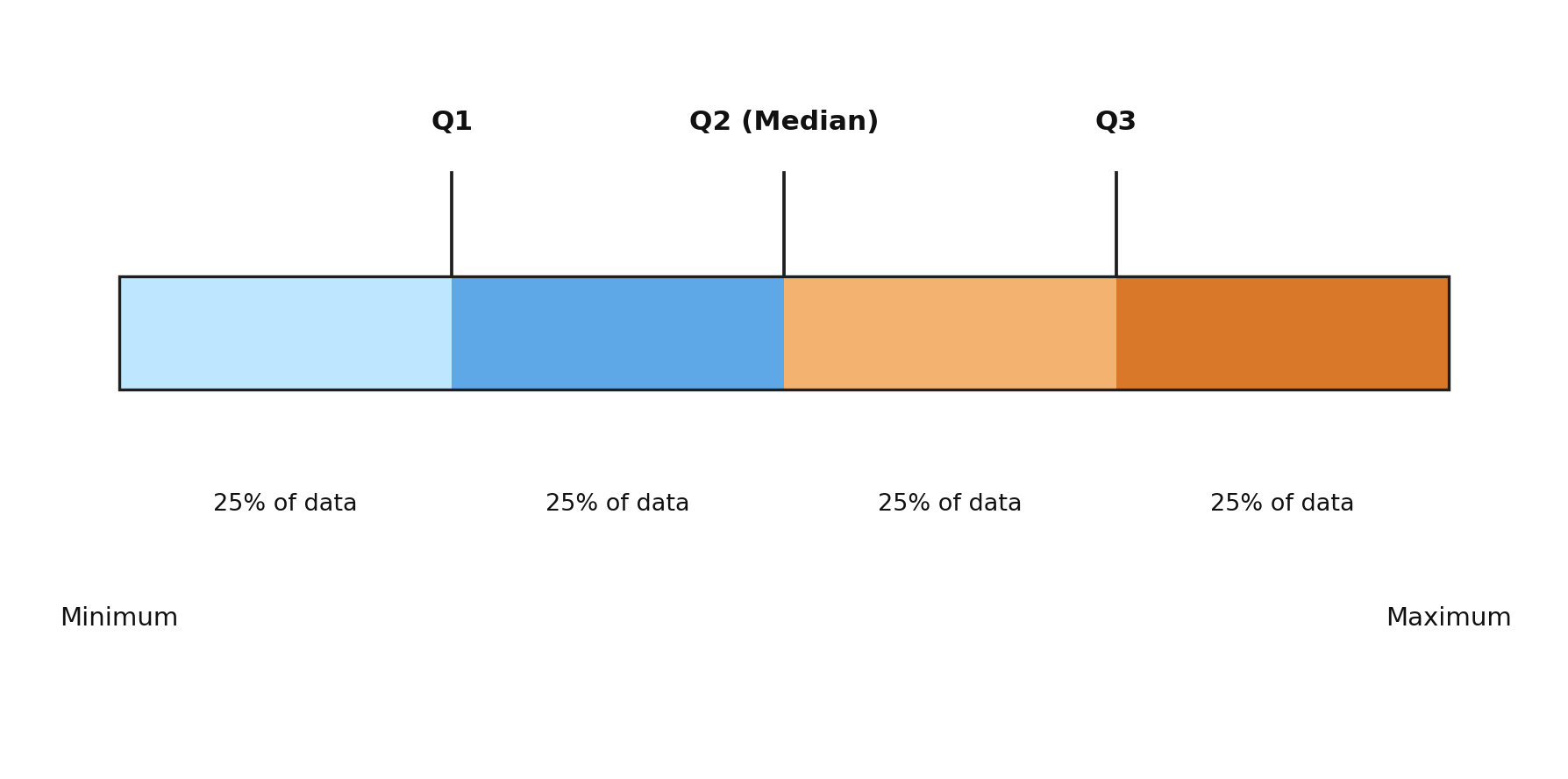
As you may recall from the previous course, the median splits an ordered dataset into two halves. Quartiles take this idea one step further. Along with the median, we identify two additional values: one that marks the middle of the lower half and one that marks the middle of the upper half. Together, these three values carve the data into four groups, each containing about one-quarter of the values.

Let's name each quartile clearly:

• Q1 (First Quartile): The median of the lower half of the data. Roughly 25% of values fall below Q1.
• Q2 (Second Quartile): The median of the entire dataset. This splits the data into two equal halves.
• Q3 (Third Quartile): The median of the upper half of the data. Roughly 75% of values fall below Q3.

Notice that Q2 is simply the median we already know how to find. The new skill in this lesson is locating Q1 and Q3 by finding the median of each half of the data.

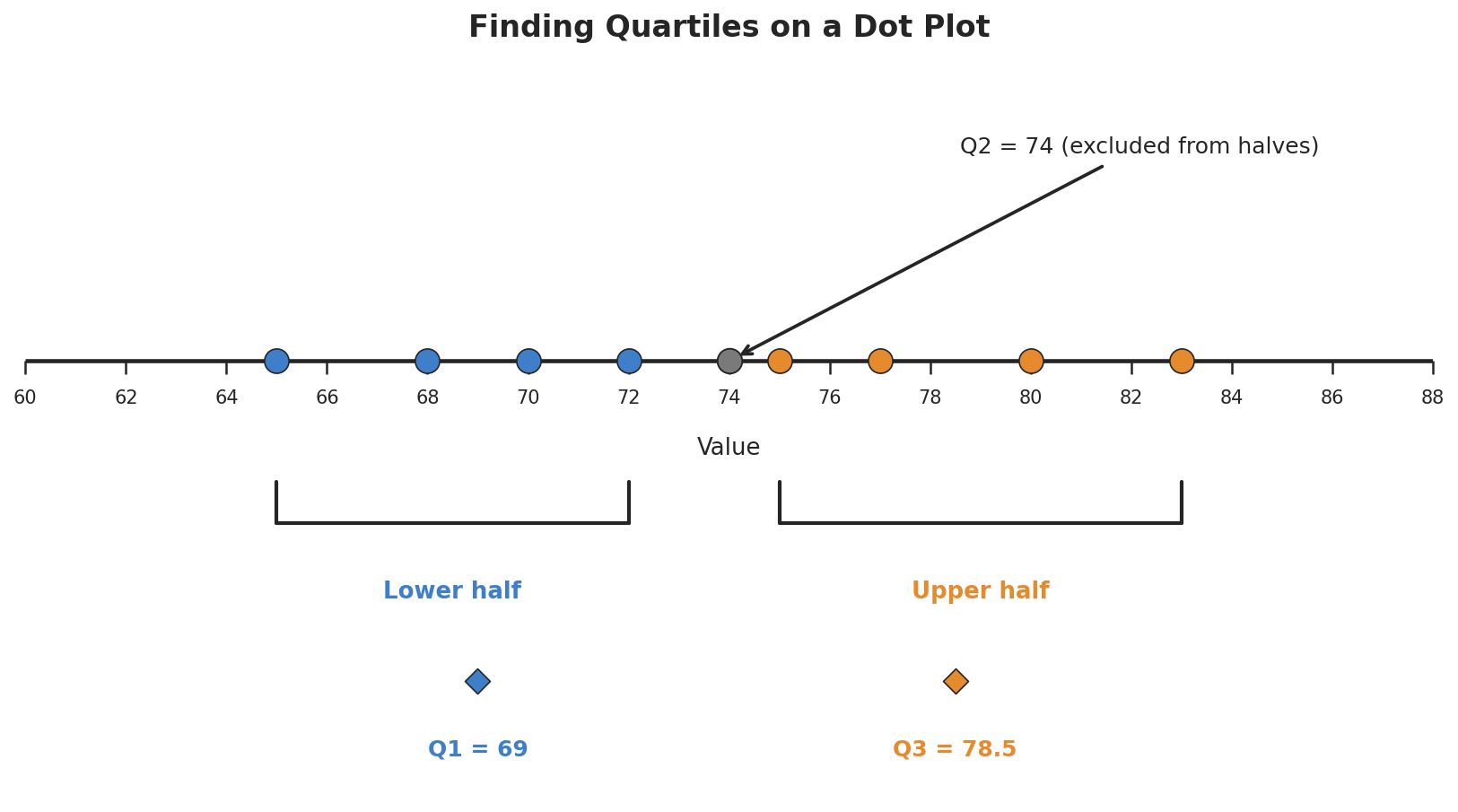
Let's walk through a complete example. Suppose we recorded the daily high temperatures (in °F) over nine days:

72, 68, 75, 80, 65, 77, 70, 83, 74

Step 1 — Order the data from least to greatest.

Step 2 — Find the median (Q2). With values, the median is the value in position . Counting to the 5th value:

The process is nearly the same when the dataset has an even number of values. The only difference is how we form the halves. Let's use a new example: the number of customer orders at a small bakery over eight days.

30, 45, 22, 38, 50, 27, 33, 41

Step 1 — Order the data.

Step 2 — Find the median (Q2). With $$ values, the median is the average of the 4th and 5th values:

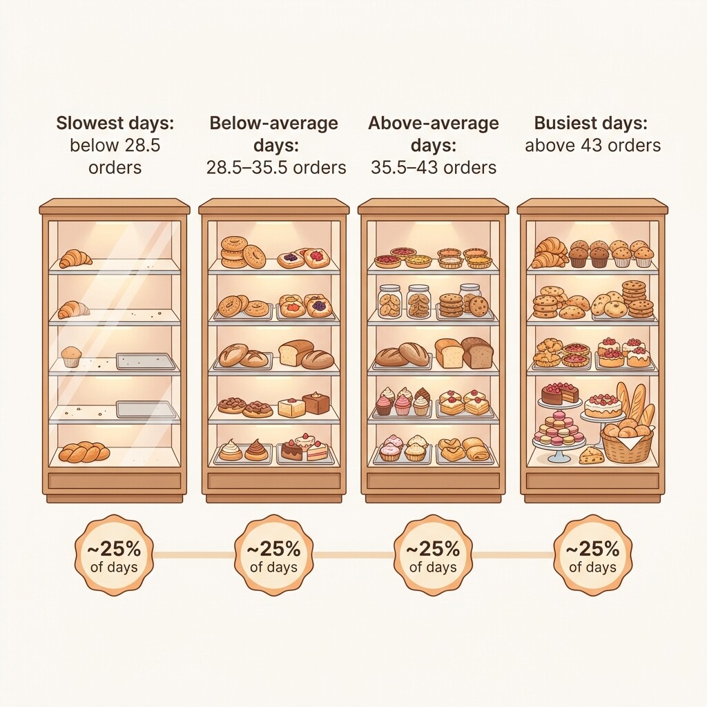
Let's step back and see what our bakery results actually mean. The three quartiles ($Q1 = 28.5$, median $= 35.5$, $Q3 = 43$) divide the eight data values into four groups of roughly two values each:

In this lesson, you learned how to find Q1, Q2 (the median), and Q3 by ordering the data, splitting it into halves, and finding the median of each half. The key difference between odd and even datasets is that an odd-sized set excludes the median from both halves, while an even-sized set splits neatly into two equal groups. Together, these three quartiles divide a dataset into four roughly equal parts, giving us a much more detailed view of spread than the range alone.

Now it is time to put these steps into action! The practice exercises ahead will guide you from a scaffolded walkthrough all the way to finding quartiles independently in real-world scenarios. Once you feel confident with quartiles, the next lesson will show you how to use Q1 and Q3 to calculate the interquartile range (IQR) — a powerful measure of spread that focuses on the middle 50% of your data.