Welcome back to Measuring Spread and Variability! This is lesson three of four, which means we are almost done with this course. So far, we have measured spread using the range and learned how to locate Q1, Q2 (the median), and Q3 to divide a dataset into four roughly equal groups. Now it is time to put those quartile skills to work. In this lesson, we will calculate and interpret the interquartile range (IQR) — a measure of spread that zeroes in on the middle 50% of the data and ignores the extremes.

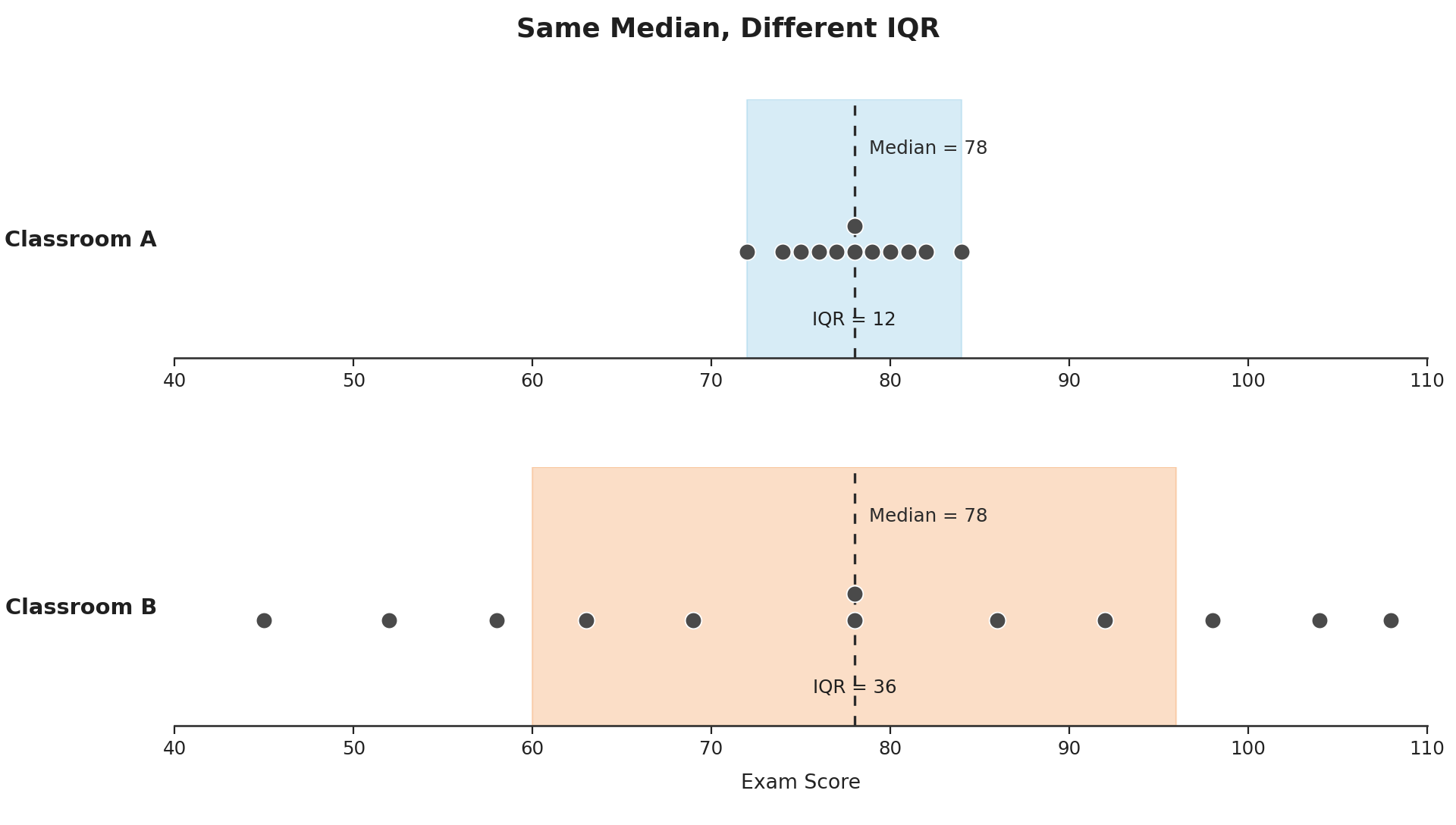
Imagine two classrooms that both scored a median of 78 on an exam. In Classroom A, the middle half of scores runs from 72 to 84. In Classroom B, the middle half stretches from 60 to 96. Even though both classes share the same center, the experience of teaching them would feel very different because Classroom B has far more variability among its students.

The interquartile range gives us a single number to capture exactly this kind of difference. By measuring only the span of the middle 50%, we get a sense of how tightly or loosely the "typical" values are clustered — without being thrown off by a few unusually high or low scores.

As you may recall from the previous lesson, Q1 marks the boundary below which roughly 25% of the data falls, and Q3 marks the boundary below which roughly 75% falls. The interquartile range is simply the distance between these two values:

That's it — one subtraction is all it takes. The IQR tells us the width of the interval that contains the middle 50% of our data. A smaller IQR means the middle values are bunched closely together, while a larger IQR means they are more spread out.

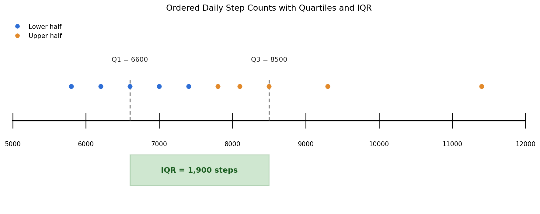
Let's put the formula into practice with a real-world scenario. Suppose we tracked daily step counts over ten days:

6,200   7,400   8,100   5,800   9,300   7,000   8,500   6,600   7,800   11,400

Step 1 — Order the data.

A number by itself only tells part of the story. The IQR becomes truly useful when we tie it back to the situation at hand. Consider our step-count example: an IQR of 1,900 out of a median around 7,600 suggests moderate day-to-day consistency. If the IQR had been only 400, we would say our daily activity was very steady. If it had been 4,000, we would say our routine varied quite a bit from one day to the next.

When writing or speaking about the IQR, always connect the number to the real-world context. Saying "the IQR is 1,900" is correct but incomplete. Saying "the middle half of daily step counts spans about 1,900 steps" paints a picture that is much easier to understand.

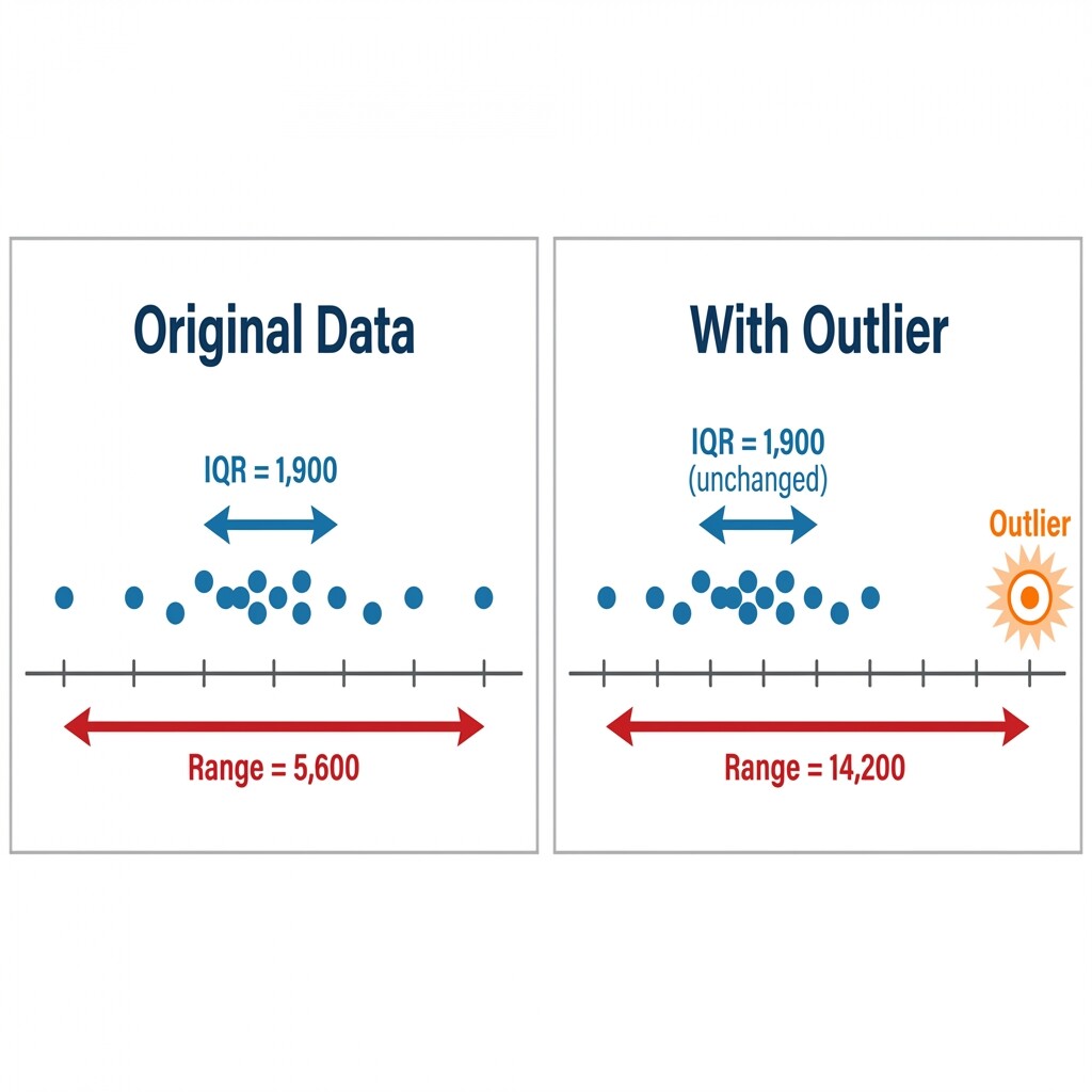
Recall from our first lesson that the range uses only the minimum and maximum, which makes it sensitive to extreme values. Let's see what happens to our step-count data if the highest value, 11,400, had actually been 20,000 — perhaps we hiked a mountain that day.

• Range before: $11400 - 5800 = 5600$
• Range after: $20000 - 5800 = 14200$

The range more than doubled! Now let's check the IQR. Since 20,000 replaces 11,400 in the upper half, Q3 is still the 3rd value of that half: $$. Q1 has not changed either. So:

In this lesson, we learned how to calculate the interquartile range using the formula $IQR = Q3 - Q1$ and explored what this number actually means. The IQR describes the spread of the middle 50% of a dataset, giving us a focused view of how much the typical values vary. We also saw that, unlike the range, the IQR is not influenced by extreme values, making it a dependable summary of spread in real-world data. In the next and final lesson, we will put the range and IQR side by side to compare what each measure reveals and when each is most useful.

For now, it is time to practice! The exercises ahead will walk you through IQR calculations, dataset comparisons, and real-life interpretation in contexts like coffee shop sales and household budgets — so let's jump in and make these skills your own.