Welcome to Measuring Spread and Variability, the second course in this learning path! In the previous course, we explored how to summarize a dataset with measures of center like the mean, median, and mode. Those tools help us describe a "typical" value, but they only tell half the story. Two datasets can share the exact same mean yet look completely different. What's missing? A way to describe how much the values spread out. That is exactly what this course is about, and in this first lesson we will introduce the concept of variability and learn our first tool for measuring it: the range.

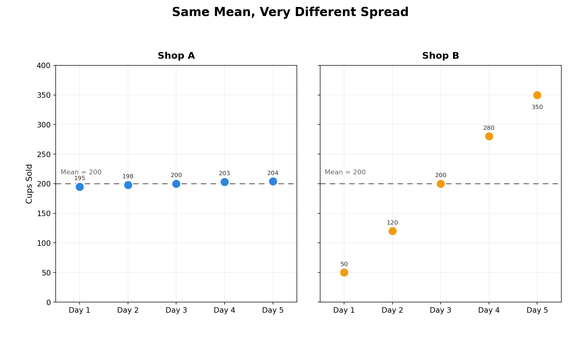
Imagine two coffee shops that each sell an average of 200 cups per day. At Shop A the daily counts over a week are 195, 198, 200, 203, 204. At Shop B they are 50, 120, 200, 280, 350. The mean is 200 in both cases, but the day-to-day experience at each shop is very different. Shop A is remarkably steady, while Shop B swings wildly from slow days to extremely busy ones.

This difference is what we call variability (sometimes called spread). Variability tells us how much the individual data values differ from one another. High variability means the values are scattered over a wide area; low variability means they cluster tightly together. Recognizing variability is essential whenever we want to understand not just what is typical, but how consistent or unpredictable the data really are.

The simplest way to quantify spread is the range. The range captures the total span of a dataset in a single number:

That's it — find the largest value, find the smallest value, and subtract. Let's apply this to our coffee shop example:

• Shop A: Maximum $= 204$, Minimum $= 195$, so Range cups.

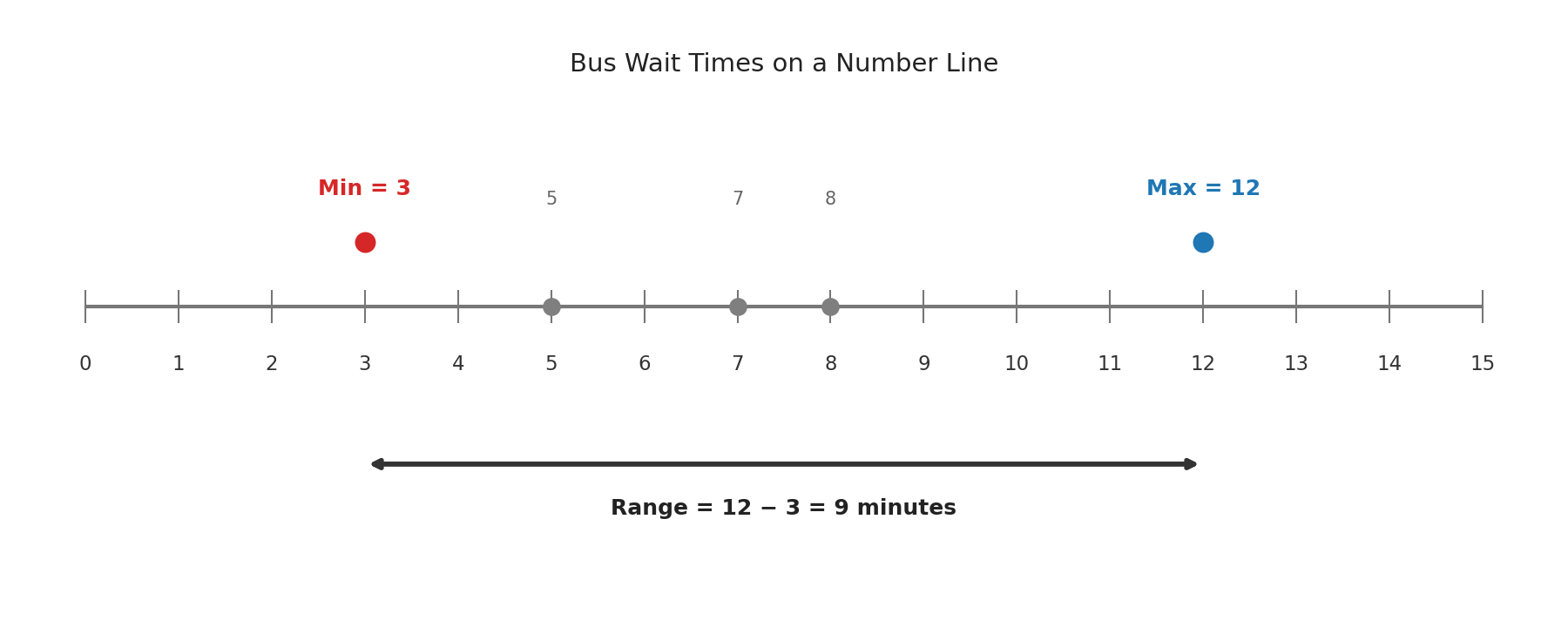
Suppose we recorded the number of minutes a commuter waited for the bus on five different mornings: 3, 12, 7, 5, 8. Here is how to find the range:

1. Identify the maximum. Scan the values: the largest is $12$.
2. Identify the minimum. The smallest is $3$.
3. Subtract. $\text{Range} = 12 - 3 = 9$ minutes.

The range tells us that the gap between the shortest wait and the longest wait was . Notice that we do not need to sort the data or compute an average — we only need two values: the highest and the lowest.

The range is quick to calculate and easy to interpret, which makes it a great first look at variability. However, it has an important limitation: it depends on only the two most extreme values and ignores everything in between.

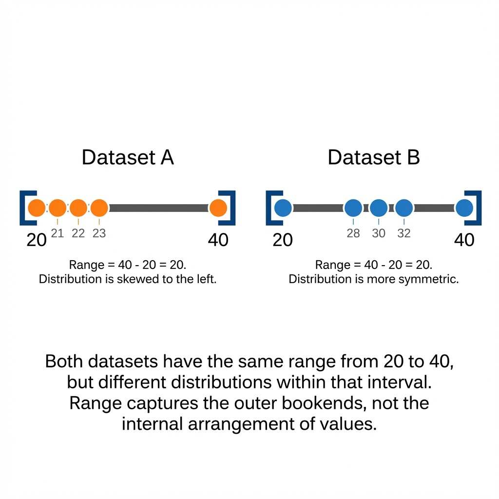
Consider two datasets of daily commute times (in minutes):

Both datasets have a range of 20, yet they tell very different stories. In Dataset A, most commutes are tightly packed near 20 minutes with one unusually long trip. In Dataset B, the values are spread more evenly across the interval. Because the range cannot distinguish these two patterns, we will need additional measures of spread — like quartiles and the interquartile range — in the lessons ahead.

In this lesson you learned that variability describes how much data values differ from one another, and you practiced calculating the range as $\text{Maximum} - \text{Minimum}$. The range gives us a fast snapshot of overall spread, but because it relies on only the two extreme values, it can miss important details about how the rest of the data are distributed.

Up next, you will put these ideas into practice with exercises that ask you to compare variability between datasets and compute the range in real-world scenarios. In future lessons, we will go deeper with quartiles and the interquartile range to capture what the range leaves out — but first, head into the practice tasks and see how well you can spot and measure variability on your own!