In the previous lesson, you created your first Grafana dashboard with two panels: a time series chart showing CPU usage trends over time and a stat visualization displaying the average memory usage as a single number. These two visualization types work great for certain monitoring questions — time series helps you see how metrics change over time, while stat gives you a quick summary value at a glance.

However, monitoring systems involves asking many different types of questions about your data. Sometimes, you need to compare average values across multiple hosts to identify which one is consuming the most resources. Other times, you need to see if a current value has crossed into a dangerous threshold zone. You might want to understand how disk space is distributed across different mount points, or you might need to see raw, detailed records for troubleshooting.

Each of these questions requires a different visualization type, and each visualization type expects your query to return data in a specific structure. In this lesson, you'll learn four additional visualization types that complement the time series and stat panels you already know: bar charts for comparing aggregated values, gauges for showing current values with color-coded thresholds, pie charts for displaying proportional distributions, and tables for presenting detailed multi-column data. By the end of this lesson, you'll be able to choose the right visualization for each monitoring question you need to answer.

Let's start with a common monitoring scenario: you want to know which of your hosts is consuming the most CPU on average. A time series chart would show you trends over time, but what you really want is a simple side-by-side comparison. This is where bar charts excel.

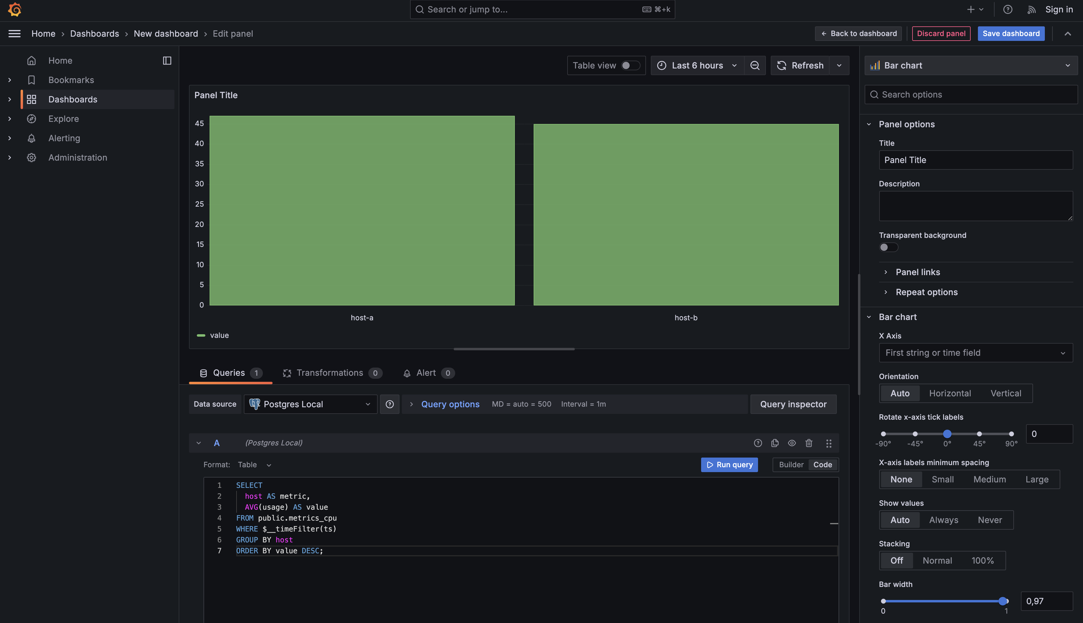
To create a bar chart, add a new visualization to your dashboard and enter this query:

Notice how this query differs from the time series query you wrote in the previous lesson. You're still using $__timeFilter(ts) to respect the dashboard's time range, but you're not using $__time(ts) at all. That's because you're not plotting values over time — you're calculating a single aggregated value for each host.

The GROUP BY host clause creates one result row per host, and AVG(usage) calculates the average CPU usage for that host across the selected time period. The metric and value column aliases follow Grafana's convention, just like in time series queries, but here they mean something different. The metric column determines which bars appear on your chart (one bar per host), and the value column determines the height of each bar.

By ordering the results with ORDER BY value DESC, you ensure the hosts with the highest CPU usage appear first, making it easy to spot problem hosts immediately.

Sometimes, you need to monitor a single metric and know immediately whether it's in a safe, warning, or critical state. For example, you might want to display the current disk usage for your root mount point with visual indicators showing when it's approaching capacity. This is exactly what gauge visualizations are designed for.

Add another panel to your dashboard and enter this query:

This query is structured very differently from both the time series and bar chart queries. You're filtering down to one specific item (host-a's root mount point) and then using ORDER BY ts DESC LIMIT 1 to retrieve only the most recent measurement. The result is a single number representing the current disk usage percentage.

The value column tells Grafana exactly which number to display on the gauge. Since this query returns only one row, Grafana reads it as the "current value" of the metric.

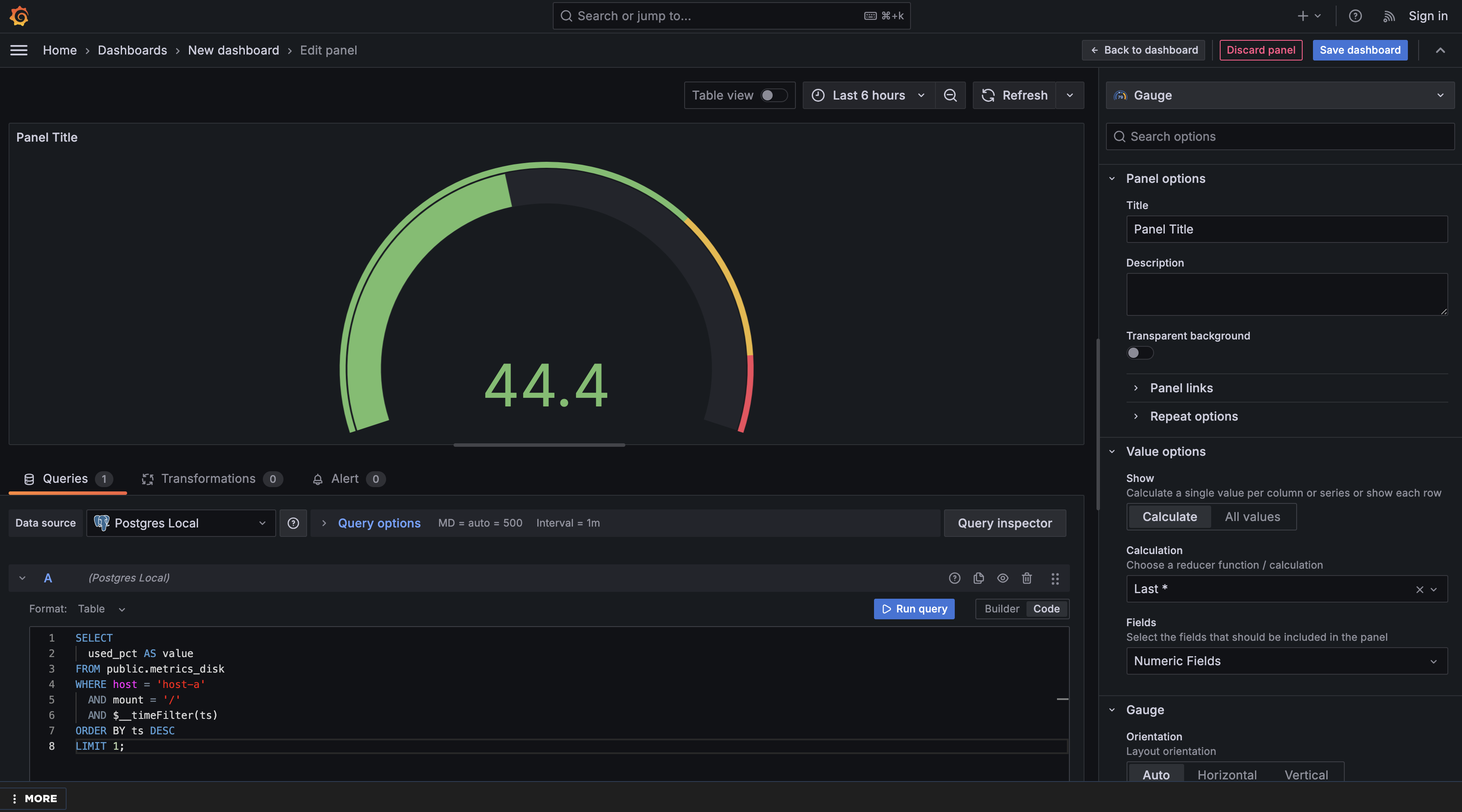
After running the query, switch the visualization type to Gauge. You'll need to configure a few settings to tell Grafana how to interpret your single value:

Configure Value Options:

• Under Value options → Show, choose Calculate (since your query returns one row, and you want that single number displayed)
• Under Value options → Calculation, keep Last selected (to display the latest value from your result)
• Under Value options → Fields, choose Numeric Fields (so Grafana uses the value column for the gauge)

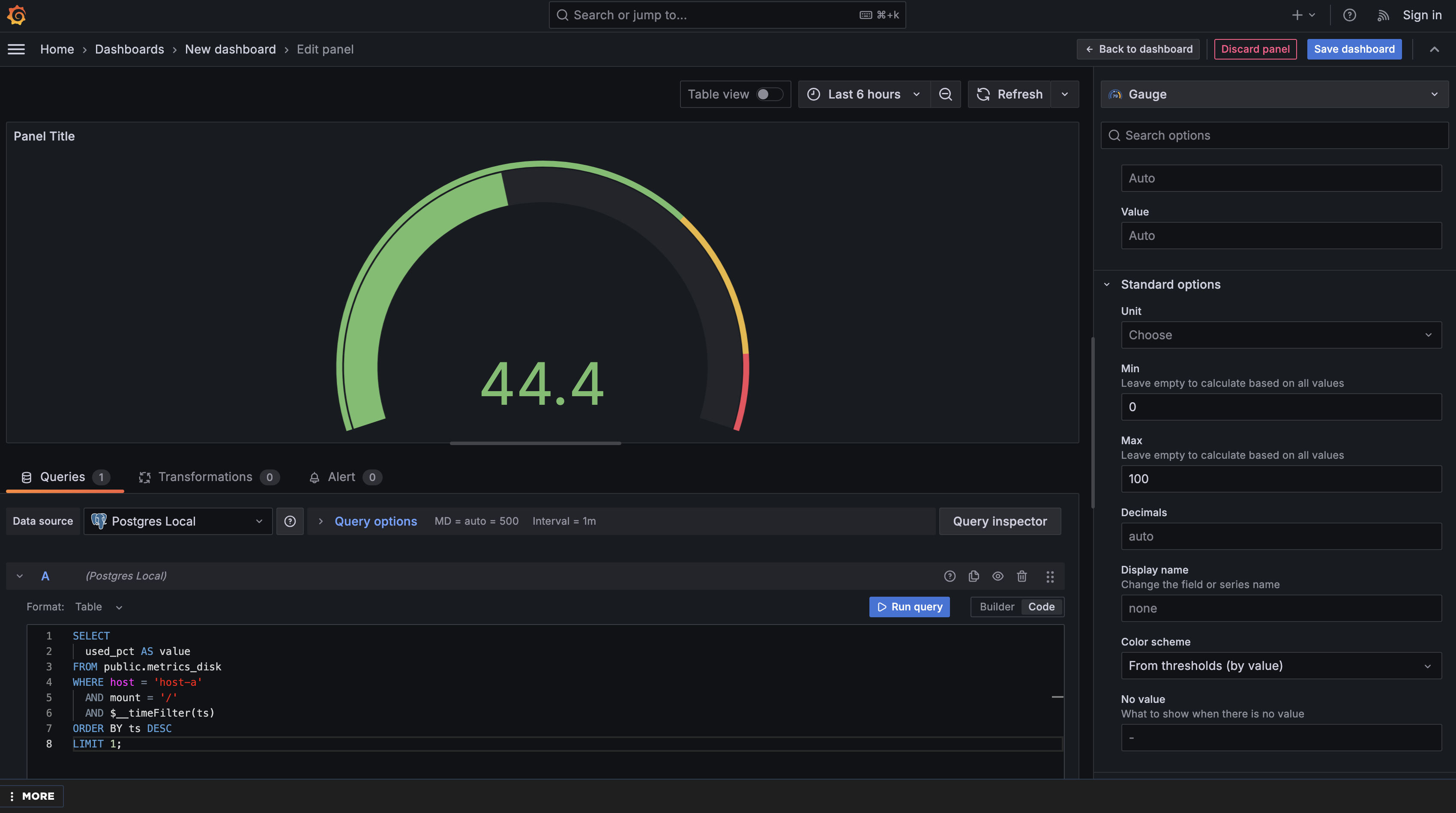
Set the Gauge Range: Under Standard options, set Min to 0 and Max to 100 (since disk usage is measured as a percentage). This tells the gauge what the full possible range of values is, so it can position the needle correctly.

Without setting these values explicitly, Grafana would auto-scale the gauge based on your current data. For example, if your disk is currently at 45% usage, Grafana might automatically create a gauge from 0 to 50, making 45% appear near the top — which would be misleading. By fixing the range at 0–100, you ensure that 50% always appears in the middle of the gauge, 75% appears three-quarters of the way up, and 90% appears near the top. This consistency is critical for at-a-glance interpretation — team members can instantly recognize the severity of a value because the visual position remains meaningful across different readings.

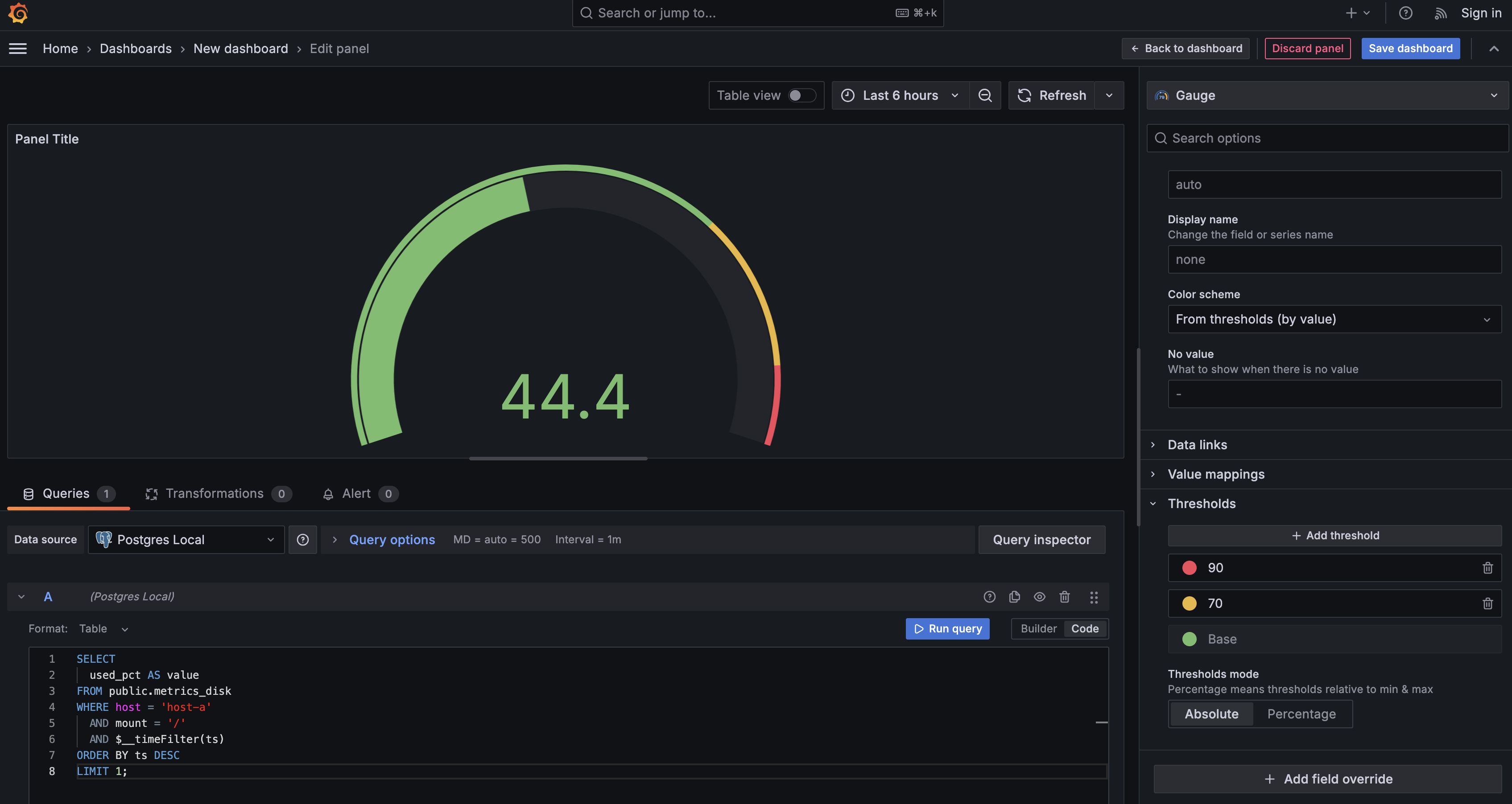
Once applied, you'll see a gauge displaying the current disk usage. Now you can configure threshold ranges to highlight severity levels. Under Thresholds, set up color-coded ranges:

• 0–70% (green): healthy
• 70–90% (yellow): warning
• 90–100% (red): critical

This makes the gauge a powerful at-a-glance indicator. Team members can instantly interpret system health based on color and needle position. They don't need to analyze multiple values or time series — the visual representation tells the story immediately.

Gauges are ideal for metrics where real-time thresholds matter, such as disk usage, memory pressure, CPU saturation, service latency, or error rates. Whenever you need to answer the question "Is this value currently in a safe range?" a gauge provides the fastest, clearest answer.

When you need to understand how a total is divided among different parts, pie charts provide an intuitive visualization. For instance, you might want to see how disk space is distributed across different mount points on a single host. While a bar chart could show this as well, a pie chart emphasizes the proportional relationship — how each part contributes to the whole.

Create a new panel with this query:

This query structure looks similar to the bar chart query because both are creating categories for comparison. You're grouping by mount to create one result row per mount point and calculating the average disk usage percentage for each. The difference is in how you'll visualize the results.

The metric column (mount point names) determines what slices appear in your pie chart, and the value column (average usage percentage) determines the size of each slice. By filtering to a single host with WHERE host = 'host-a', you ensure the pie chart shows the complete picture for one machine rather than mixing data from multiple hosts.

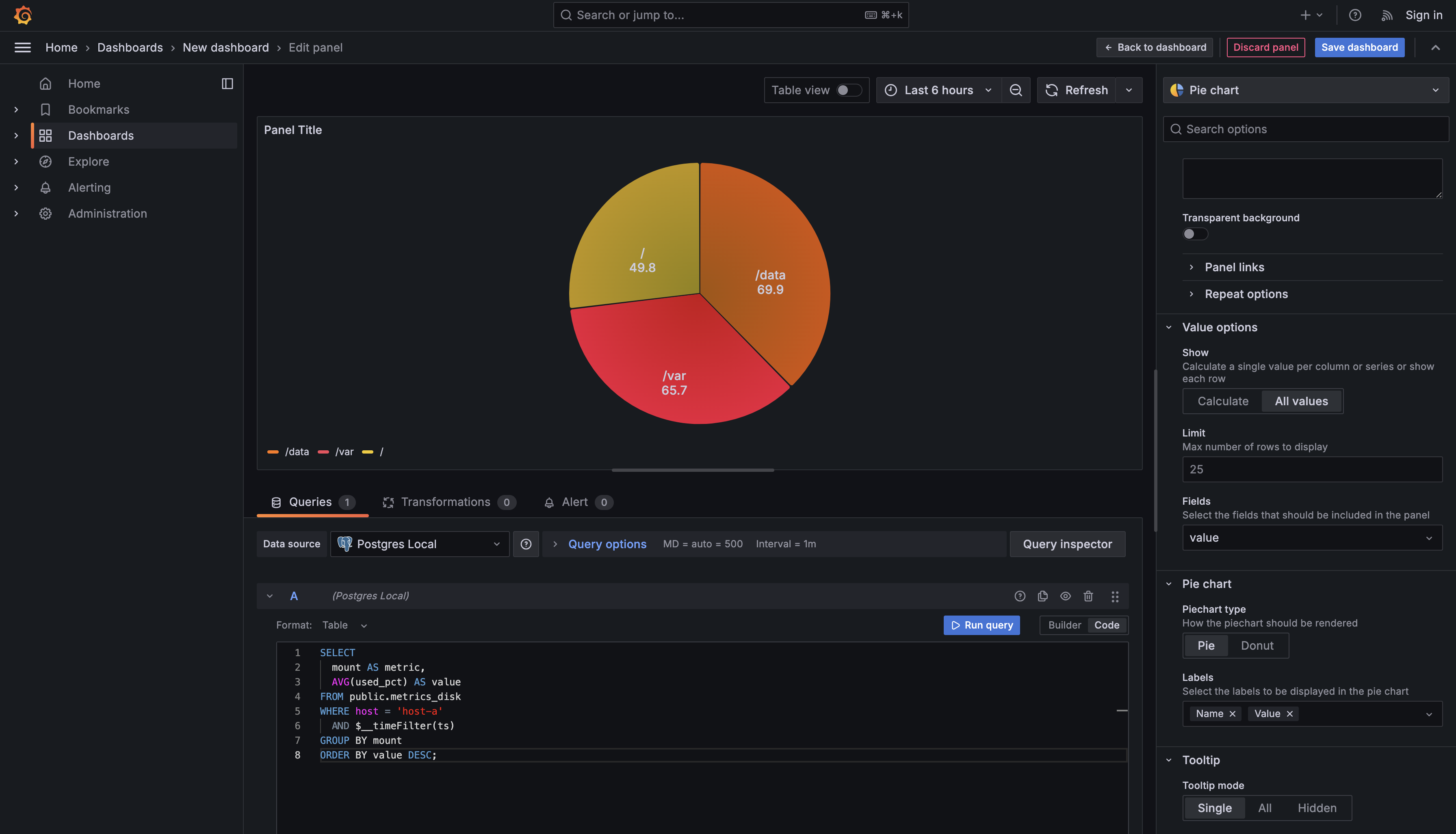
After running the query, switch the visualization type to Pie chart. Then configure the panel so Grafana uses your columns correctly:

• Under Value options → Show, choose All values so each mount point becomes its own slice.
• Under Value options → Fields, select value to use the numeric column for slice size.
• Under Pie chart → Labels, select Name and Value to display the mount point names and values as slice labels.

With these settings applied, you’ll see a circular chart divided into colored slices, each representing one mount point. The size of each slice corresponds to that mount point’s disk usage percentage. Larger slices immediately stand out, helping you identify which mount points are consuming the most space.

All the visualizations you've learned so far focus on presenting data graphically, but sometimes you need to see the actual raw records with all their details. This is especially useful for troubleshooting or when you need to drill into specific values. Tables give you this detailed view.

Add one more panel with this query:

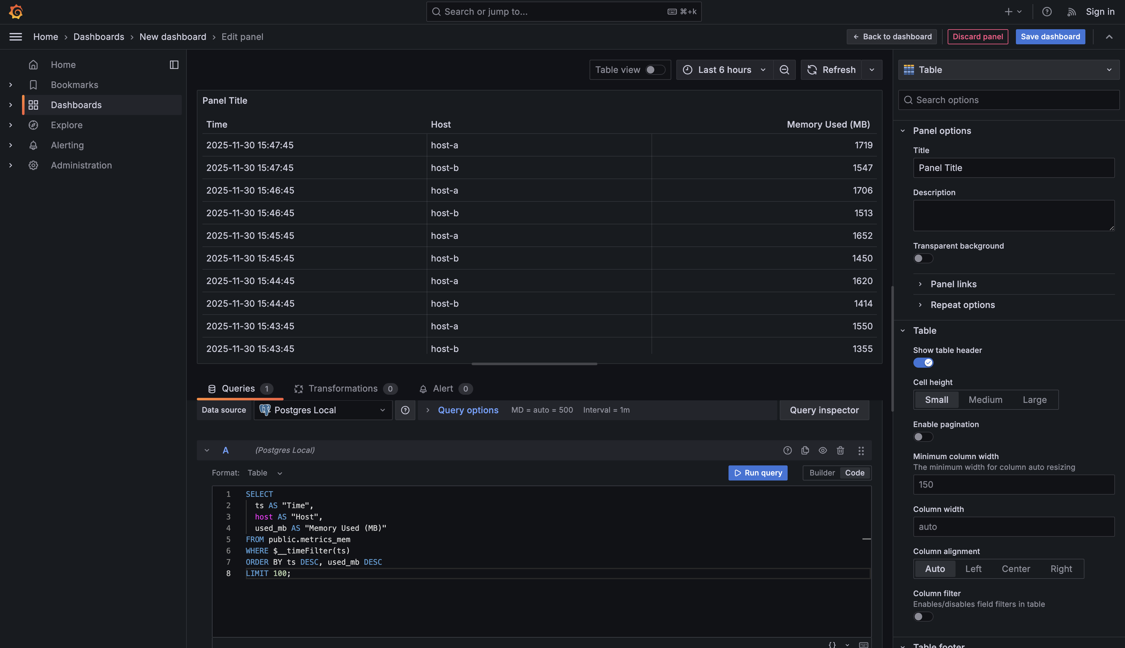
This query returns multiple columns of data, and each column will become a column in your table. Notice the use of column aliases with quotes like AS "Time" and AS "Host". These aliases become the column headers in your table, so you're writing them in a readable format with proper capitalization and spacing.

The query selects three pieces of information for each memory measurement: the timestamp, which host it came from, and how much memory was used in megabytes. By ordering with ORDER BY ts DESC, used_mb DESC, you ensure the most recent records appear first, and within each timestamp, the highest memory consumers appear at the top. The LIMIT 100 clause keeps your table from becoming overwhelming by restricting it to the 100 most relevant rows.

Change the visualization type to Table. Unlike the graphical visualizations you've been using, the table will display your data in rows and columns, similar to a spreadsheet. Each row represents one measurement record, and each column shows a different attribute of that measurement.

Tables are particularly valuable when you need to see exact values rather than trends or comparisons. For example, if you notice a memory spike in a time series chart, you might add a table panel to see exactly which hosts experienced high memory usage and at what specific times. The tabular format also makes it easy to identify patterns across multiple dimensions simultaneously — you can see which hosts consistently appear among the top memory consumers or notice if certain times of day show higher usage.

You've now learned six different visualization types that work together to create comprehensive monitoring dashboards. Time series charts track how metrics change over time, while stat panels display single summary values at a glance. Bar charts let you compare aggregated values across categories like hosts or services. Gauges show current values with color-coded thresholds for immediate status assessment. Pie charts reveal proportional distributions when you need to understand how a total is divided. Tables present detailed multi-column data for troubleshooting and detailed analysis.

Each visualization type requires a specific query structure. Time series queries use $__time(ts) to identify the time dimension and return metric-value pairs over time. Bar and pie charts use GROUP BY with aggregation to create categories for comparison, without the time dimension. Gauges return a single latest value by filtering to one item and using ORDER BY ts DESC LIMIT 1. Tables return multiple columns with readable aliases to create spreadsheet-like views of raw data. Despite these differences, all queries still use $__timeFilter(ts) to respect your dashboard's time range controls, ensuring consistency across panels.

In the upcoming practice exercises, you'll add all four of these new visualization types to your dashboard: a bar chart comparing CPU usage across hosts, a gauge showing current disk usage with thresholds, a displaying disk space distribution across mount points, and a listing top memory consumers. By combining these different visualization types on a single dashboard, you'll be able to answer multiple monitoring questions at once — seeing both the big-picture trends and the detailed specifics.