Evaluating K-means Clustering

Welcome back! In this lesson, we're seeking a more in-depth understanding of the K-means clustering algorithm by using a straightforward 2D dataset. We'll explore its implementation and evaluate its performance using a well-known measure of clustering accuracy: the Rand Index.

Now that we have learned about the Rand Index and Adjusted Rand Index, it's also beneficial to familiarize ourselves with some of the R packages that provide similar functionality. The mclust package in R offers the function adjustedRandIndex, which computes the Adjusted Rand Index for comparing two clusterings.

The adjustedRandIndex function takes two vectors as input: the true labels and the predicted cluster labels. It returns a numeric value representing the Adjusted Rand Index, which ranges from -1 (no agreement) to 1 (perfect agreement), with 0 indicating random labeling.

Here is how you can use the adjustedRandIndex function in R:

# Install mclust if not already installed
# install.packages("mclust")
library(mclust)

# Calculate the Adjusted Rand Index
ari <- adjustedRandIndex(true_labels, predicted_labels)

print(paste("Adjusted Rand Index:", ari))

In the above snippet, we load the mclust package and use adjustedRandIndex to compute the Adjusted Rand Index. The inputs to the function are the true labels and the labels predicted by K-means. The function returns a numeric value representing the Adjusted Rand Index of the predicted clusters.

Just like in the Rand Index calculation, a higher Adjusted Rand Index means that our K-means algorithm has done a great job clustering.

With all the pieces at hand, let's put everything together. We'll perform K-means clustering on our toy dataset using R's kmeans function, then evaluate the results using the Adjusted Rand Index from the mclust package. We'll also visualize the clusters and their centers using ggplot2 for a more modern and flexible plotting approach.

First, we initialize the data and perform clustering:

# Load required packages
# install.packages("mclust") # Uncomment if not already installed
# install.packages("ggplot2") # Uncomment if not already installed
library(mclust)
library(ggplot2)

set.seed(42)

# Define a 2D dataset and true labels for assessment
features <- matrix(c(
  1, 1, 1, 2, 2, 1, 2, 2, 
  5, 5, 5, 6, 6, 5, 6, 6, 
  9, 9, 9, 10, 10, 9, 10, 10,
  10, 2, 10, 3, 11, 2, 11, 3, 
  4, 8, 4, 9, 5, 8, 5, 9, 
  3, 5, 3, 6, 3, 5, 3, 6
), ncol = 2, byrow = TRUE)

true_labels <- c(
  0, 0, 0, 0, 1, 1, 1, 1, 
  2, 2, 2, 2, 0, 0, 0, 0, 
  1, 1, 1, 1, 2, 2, 2, 2
)

# Perform K-means clustering
kmeans_result <- kmeans(features, centers = 3, nstart = 10)

# Obtain the predicted labels
predicted_labels <- kmeans_result$cluster

Now let's calculate the Adjusted Rand Index using mclust and print the results:

# Calculate the Adjusted Rand Index
ari <- adjustedRandIndex(true_labels, predicted_labels)

# Output the resulting cluster labels, centroids, and Adjusted Rand Index
print(paste("Cluster labels:", paste(predicted_labels, collapse = ", ")))
print("Centroids:")
print(kmeans_result$centers)
print(paste("Adjusted Rand Index:", ari))

Example output:

[1] "Cluster labels: 3, 3, 3, 3, 3, 1, 1, 1, 1, 1, 1, 1, 2, 2, 2, 2, 1, 1, 1, 1, 3, 3, 3, 3"
[1] "Centroids:"
       [,1]     [,2]
1  6.636364 8.090909
2 10.500000 2.500000
3  2.555556 3.666667
[1] "Adjusted Rand Index: 0.253832442067736"

Visualizing the clusters and centroids using ggplot2:

# Prepare data for ggplot2
df <- as.data.frame(features)
colnames(df) <- c("X1", "X2")
df$Cluster <- as.factor(predicted_labels)

centers <- as.data.frame(kmeans_result$centers)
colnames(centers) <- c("X1", "X2")

# Plot using ggplot2
plot <- ggplot(df, aes(x = X1, y = X2, color = Cluster)) +
  geom_point(size = 3) +
  geom_point(data = centers, aes(x = X1, y = X2), 
             color = "red", shape = 4, size = 6, stroke = 2) +
  labs(title = "Clusters with Centroids (Red X)", x = "X1", y = "X2") +
  theme_bw()

Output:

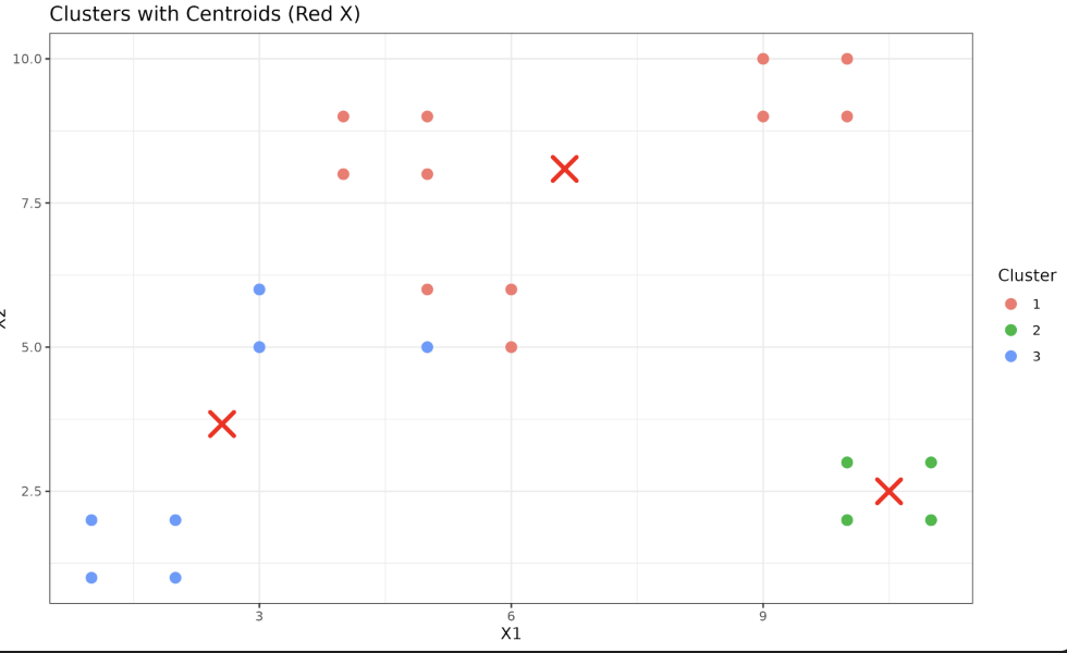
Here, we have effectively encapsulated our prior discussions on implementing K-means clustering, applying the Adjusted Rand Index, and bringing the insights to life through visual representations. R's kmeans function simplifies the K-means process into merely defining the model, fitting it to the data, and performing evaluations. By reflecting this streamlined process, the code highlights the importance of understanding essential concepts, navigating packages, and connecting functions to their origins.

The exploration of the K-means algorithm and the proper use of the Rand Index and Adjusted Rand Index has provided us with significant insights in the realm of unsupervised learning. The next phase will involve practical applications, cementing your understanding of these crucial concepts. Your understanding of these concepts, like the K-means algorithm that we discussed, will improve through multiple iterations. Happy practicing!