Choosing Clusters and Centroids

Introduction

Greetings! Our journey into K-means clustering deepens as we explore two crucial elements: the selection of the number of clusters and the initialization of centroids. Our aim is to comprehend these aspects and put them into action using R. Let's move forward!

Choosing Clusters and Initializing Centroids in K-means

The K in K-means signifies the number of clusters. Centroids, the centers of each cluster, are equally significant. Their initial placement in K-means is crucial. Poorly initialized centroids can lead to suboptimal clustering — which is why multiple runs with different initial placements are essential. This highlights the importance of choosing both the number of clusters and their initial centroids.

Revising K-means Algorithm

R’s built-in kmeans() function allows us to specify the number of clusters and also to set the initial centroids manually. Let’s see how we can do this in R using ggplot2 for visualization.

R
library(ggplot2)

# Load the iris dataset
data(iris)
iris_data <- as.matrix(iris[, 1:4])

# Set the number of clusters
num_clusters <- 3

# Randomly select initial centroids from the data
set.seed(42)
initial_centroids_idx <- sample(1:nrow(iris_data), num_clusters)
initial_centroids <- iris_data[initial_centroids_idx, ]

# Run kmeans with user-specified initial centers
kmeans_result <- kmeans(iris_data, centers = initial_centroids, iter.max = 100, nstart = 1)

# Extract cluster assignments and centroids
labels <- as.factor(kmeans_result$cluster)
centroids <- as.data.frame(kmeans_result$centers)

# Prepare data for ggplot
iris_plot <- as.data.frame(iris_data)
iris_plot$Cluster <- labels

# Visualization (using first two features for simplicity)
p_iris <- ggplot(iris_plot, aes(x = Sepal.Length, y = Sepal.Width, color = Cluster)) +
  geom_point(size = 2) +
  geom_point(data = centroids, aes(x = Sepal.Length, y = Sepal.Width), 
             color = "red", shape = 4, size = 5, stroke = 2) +
  labs(title = "K-means Clustering", x = "Sepal.Length", y = "Sepal.Width") +
  theme_bw()

The iter.max parameter in the kmeans() function controls the maximum number of iterations the algorithm will perform before stopping. In the example above, we set iter.max = 100 to allow the algorithm up to 100 iterations to converge. Typically, K-means converges much sooner, but setting a higher value ensures the algorithm has enough opportunity to find stable clusters, especially for more complex datasets. If the algorithm converges before reaching this limit, it will stop early. If you set iter.max too low, the algorithm might stop before finding a good solution; if you set it very high, it may just take a bit longer to run but won't affect the final result once convergence is reached.

Output:
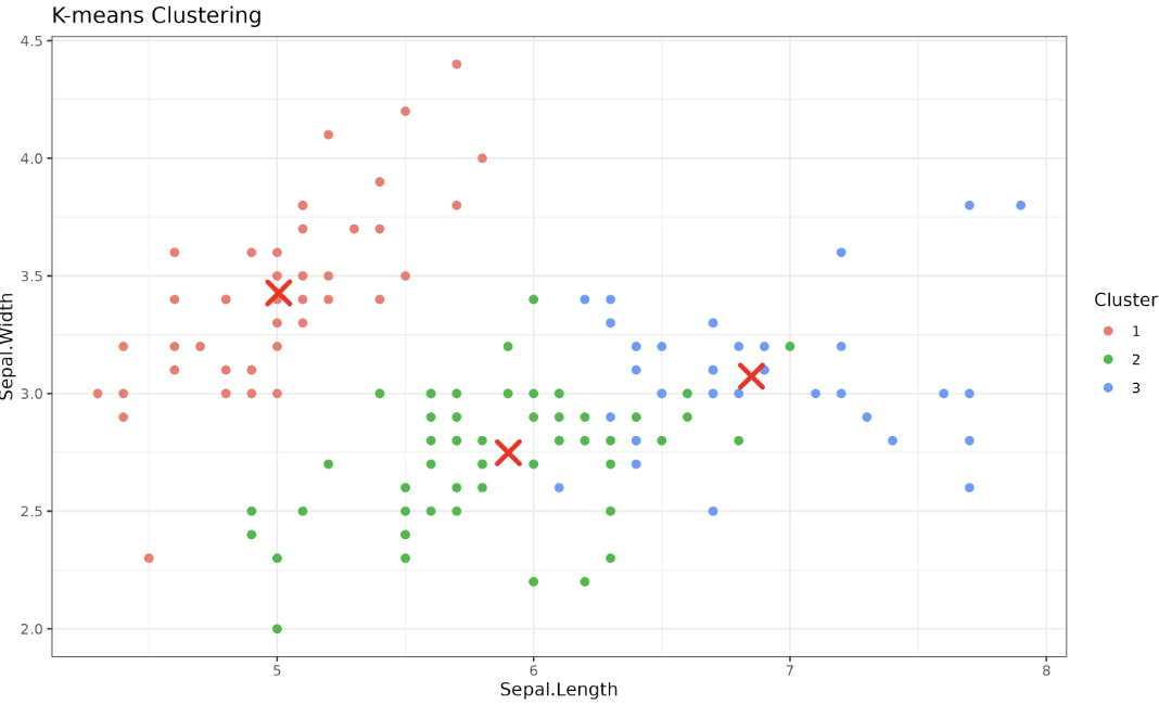
In the code above, centers is set to our chosen initial centroids, and nstart = 1 ensures that only this initialization is used. The resulting plot (assigned to p_iris) shows the data points colored by cluster, with the centroids marked in red.

Understand the Implications

As we've seen, different initial centroids and different choices for the number of clusters can lead to different results. R’s kmeans() function uses random initialization by default, which means the starting positions of the centroids are chosen randomly from the data. To reduce the risk of poor clustering due to unlucky initialization, you can use the nstart parameter to run the algorithm multiple times with different random initializations and select the best result. This helps mitigate the impact of poor initial centroid placement.

Selection of the Number of Clusters

Let’s explore how the choice of the number of clusters affects the results of K-means clustering. We’ll use a simple 2D dataset for illustration.

R
library(ggplot2)

set.seed(42)
# Create a simple 2D dataset
data <- matrix(c(3, 1, 5, 1, 2, 3,
                 8, 2, 9, 3, 7, 1,
                 15, 15, 13, 16, 14, 14), ncol = 2, byrow = TRUE)
data_df <- as.data.frame(data)
colnames(data_df) <- c("X1", "X2")

# K-means with k = 2
k2 <- kmeans(data, centers = 2, nstart = 10)
data_df$Cluster2 <- as.factor(k2$cluster)
centroids2 <- as.data.frame(k2$centers)
colnames(centroids2) <- c("X1", "X2")
centroids2$k <- "k = 2"

# K-means with k = 3
k3 <- kmeans(data, centers = 3, nstart = 10)
data_df$Cluster3 <- as.factor(k3$cluster)
centroids3 <- as.data.frame(k3$centers)
colnames(centroids3) <- c("X1", "X2")
centroids3$k <- "k = 3"

# Prepare data for combined plot
df2 <- data.frame(X1 = data_df$X1, X2 = data_df$X2, Cluster = data_df$Cluster2, k = "k = 2")
df3 <- data.frame(X1 = data_df$X1, X2 = data_df$X2, Cluster = data_df$Cluster3, k = "k = 3")
plot_df <- rbind(df2, df3)
centroids_all <- rbind(centroids2, centroids3)

# Faceted plot
p_kmeans_k <- ggplot(plot_df, aes(x = X1, y = X2, color = Cluster)) +
  geom_point(size = 2) +
  geom_point(data = centroids_all, aes(x = X1, y = X2), 
             color = "red", shape = 4, size = 5, stroke = 2, inherit.aes = FALSE) +
  labs(title = "K-means Clustering with Different k", x = "X1", y = "X2") +
  theme_bw() +
  facet_wrap(~k)

This approach uses facet_wrap() from ggplot2 to display the two clustering results side by side, without requiring any extra packages. The plot is assigned to p_kmeans_k. Here is the output:
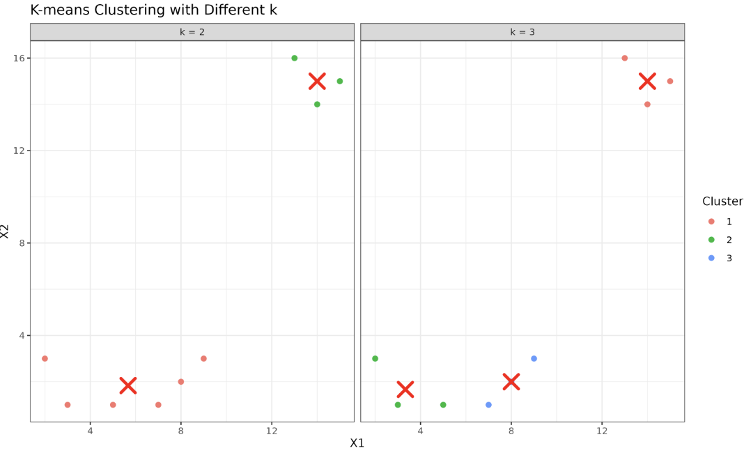
These examples illustrate the significant role the number of clusters plays in forming the final clusters. We must carefully choose this number to accurately represent the underlying structure of our data. An incorrect number of clusters could lead to overfitting or underfitting, both of which could misrepresent your data.

Initial Centroid Initialization: Potential Pitfalls and Solutions

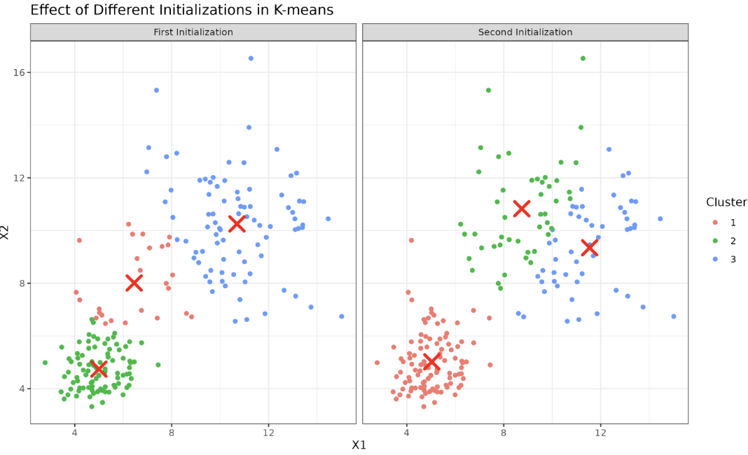
You may wonder, "Why can the initial centroid placement result in different clustering results?" The K-means algorithm is an iterative procedure that minimizes the within-cluster sum of squares. However, it only guarantees finding a local minimum, not a global one. This means that different starting positions can lead to distinct clustering outcomes.

To visualize this, imagine you're blindfolded in a hilly region where you're tasked with finding the lowest point. By feeling the ground slope, you move downward. But when there are many valleys (local minima), your starting position influences which valley (local minimum) you'll end up in — and not all valleys are equally deep. Initial centroids in K-means are akin to starting positions.

Let’s illustrate the effect of different initial centroids using a simple custom K-means implementation in R. This will help us see how sensitive the results can be to the initial choice.

R
library(ggplot2)
library(tidyr)

set.seed(0)
# Data preparation
x1 <- matrix(rnorm(200, mean = 5, sd = 1), ncol = 2)
x2 <- matrix(rnorm(200, mean = 10, sd = 2), ncol = 2)
x <- rbind(x1, x2)
colnames(x) <- c("X1", "X2")

k <- 3

# Euclidean distance function
calc_distance <- function(a, b) sqrt(sum((a - b)^2))

# Assign each point to the nearest centroid
find_closest_centroids <- function(centroids, data) {
  apply(data, 1, function(point) {
    which.min(apply(centroids, 1, function(centroid) calc_distance(point, centroid)))
  })
}

# Calculate new centroids as the mean of assigned points
calc_centroids <- function(clusters, data, k) {
  sapply(1:k, function(cluster) {
    colMeans(data[clusters == cluster, , drop = FALSE])
  })
}

# Custom K-means function
kmeans_custom <- function(data, initial_centroids, k, max_iter = 10) {
  centroids <- initial_centroids
  for (i in 1:max_iter) {
    clusters <- find_closest_centroids(centroids, data)
    centroids <- t(calc_centroids(clusters, data, k))
  }
  list(centroids = centroids, clusters = clusters)
}

# Try two different initializations
set.seed(42)
init_idx1 <- sample(1:nrow(x), k)
init_idx2 <- sample(1:nrow(x), k)
init_centroids1 <- x[init_idx1, ]
init_centroids2 <- x[init_idx2, ]

result1 <- kmeans_custom(x, init_centroids1, k)
result2 <- kmeans_custom(x, init_centroids2, k)

# Prepare data for faceted plot
df1 <- as.data.frame(x)
df1$Cluster <- as.factor(result1$clusters)
df1$Init <- "First Initialization"
centroids1 <- as.data.frame(result1$centroids)
colnames(centroids1) <- c("X1", "X2")
centroids1$Init <- "First Initialization"

df2 <- as.data.frame(x)
df2$Cluster <- as.factor(result2$clusters)
df2$Init <- "Second Initialization"
centroids2 <- as.data.frame(result2$centroids)
colnames(centroids2) <- c("X1", "X2")
centroids2$Init <- "Second Initialization"

plot_df <- rbind(df1, df2)
centroids_all <- rbind(centroids1, centroids2)

p_init <- ggplot(plot_df, aes(x = X1, y = X2, color = Cluster)) +
  geom_point(size = 1.5) +
  geom_point(data = centroids_all, aes(x = X1, y = X2), 
             color = "red", shape = 4, size = 5, stroke = 2, inherit.aes = FALSE) +
  labs(title = "Effect of Different Initializations in K-means", x = "X1", y = "X2") +
  theme_bw() +
  facet_wrap(~Init)

The plot is assigned to p_init and will display the two clustering results side by side, each corresponding to a different initialization. You can see the plot below:
Lesson Summary and Practice

In this lesson, we explored the principles of choosing the number of clusters and initializing centroids in K-means, all within the R environment. You learned how to set the number of clusters, specify initial centroids, and visualize the results using ggplot2. You also saw how different choices can affect the outcome of clustering. Practice these concepts to deepen your understanding and master K-means clustering in R.

Sign up

Join the 1M+ learners on CodeSignal

Be a part of our community of 1M+ users who develop and demonstrate their skills on CodeSignal