Distance Metrics in Clustering

What Are Distance Metrics?

Distance metrics are mathematical formulas used to measure how far apart two points are. In clustering, these metrics help us determine how similar or different data points are from each other. The choice of distance metric can significantly affect the clustering results.

Euclidean Distance: Definition and R Implementation

Distance = \sqrt{\sum_{i=1}^{n} (p_i - q_i)^2}

Manhattan Distance: Definition and R Implementation

Distance = \sum_{i=1}^{n} |p_i - q_i|

Cosine Distance: Definition and R Implementation

Similarity = \frac{A \cdot B}{||A|| \cdot ||B||}

Using Distance Metrics in Hierarchical Clustering

The distance metric you choose determines how the clustering algorithm groups data points. Let’s see how to use these metrics in a hierarchical clustering algorithm by first creating a flexible distance matrix function. Distance Matrix Function: Rcalculate_distance_matrix <- function(X, clusters, distance_metric) { n <- length(clusters) dist_matrix <- matrix(0, nrow = n, ncol = n) for (i in seq_along(clusters)) { if (is.null(clusters[[i]])) next for (j in seq_along(clusters)) { if (j <= i || is.null(clusters[[j]])) next dists <- c() for (k in clusters[[i]]) { for (l in clusters[[j]]) { dists <- c(dists, distance_metric(X[k, ], X[l, ])) } } dist_matrix[i, j] <- dist_matrix[j, i] <- mean(dists) } } return(dist_matrix) }calculate_distance_matrix <- function(X, clusters, distance_metric) { n <- length(clusters) dist_matrix <- matrix(0, nrow = n, ncol = n) for (i in seq_along(clusters)) { if (is.null(clusters[[i]])) next for (j in seq_along(clusters)) { if (j <= i || is.null(clusters[[j]])) next dists <- c() for (k in clusters[[i]]) { for (l in clusters[[j]]) { dists <- c(dists, distance_metric(X[k, ], X[l, ])) } } dist_matrix[i, j] <- dist_matrix[j, i] <- mean(dists) } } return(dist_matrix) }

Agglomerative Clustering with Custom Distance Metrics

Now, let’s use the distance matrix in an agglomerative clustering function that accepts any distance metric. Agglomerative Clustering Function: Ragglomerative_clustering <- function(X, n_clusters, distance_metric) { clusters <- lapply(1:nrow(X), function(i) i) while (length(Filter(Negate(is.null), clusters)) > n_clusters) { dist_matrix <- calculate_distance_matrix(X, clusters, distance_metric) dist_matrix[lower.tri(dist_matrix, diag = TRUE)] <- Inf min_idx <- which(dist_matrix == min(dist_matrix), arr.ind = TRUE)[1, ] idx1 <- min_idx[1] idx2 <- min_idx[2] clusters[[idx1]] <- c(clusters[[idx1]], clusters[[idx2]]) clusters[[idx2]] <- NULL } labels <- rep(NA, nrow(X)) valid_clusters <- Filter(Negate(is.null), clusters) for (label in seq_along(valid_clusters)) { for (i in valid_clusters[[label]]) { labels[i] <- label } } return(labels) }agglomerative_clustering <- function(X, n_clusters, distance_metric) { clusters <- lapply(1:nrow(X), function(i) i) while (length(Filter(Negate(is.null), clusters)) > n_clusters) { dist_matrix <- calculate_distance_matrix(X, clusters, distance_metric) dist_matrix[lower.tri(dist_matrix, diag = TRUE)] <- Inf min_idx <- which(dist_matrix == min(dist_matrix), arr.ind = TRUE)[1, ] idx1 <- min_idx[1] idx2 <- min_idx[2] clusters[[idx1]] <- c(clusters[[idx1]], clusters[[idx2]]) clusters[[idx2]] <- NULL } labels <- rep(NA, nrow(X)) valid_clusters <- Filter(Negate(is.null), clusters) for (label in seq_along(valid_clusters)) { for (i in valid_clusters[[label]]) { labels[i] <- label } } return(labels) }

Preparing the Dataset

Let’s use the Iris dataset and scale it for clustering. R library(datasets) library(scales) dataset <- as.matrix(iris[, 1:4]) dataset <- scale(dataset) library(datasets) library(scales) dataset <- as.matrix(iris[, 1:4]) dataset <- scale(dataset) Scaling the data before clustering is important because some distance metrics, like Euclidean and Manhattan, are sensitive to the scale of the variables. If features are measured on different scales, those with larger ranges can dominate the distance calculations, leading to biased clustering results. Scaling ensures that each feature contributes equally to the distance computation. In contrast, cosine distance is less affected by the scale of the variables, as it measures the angle between vectors rather than their magnitude.

Clustering with Different Distance Metrics

Now, cluster the data using each distance metric. R n_clusters <- 3 labels_euc <- agglomerative_clustering(dataset, n_clusters, euclidean_distance) labels_man <- agglomerative_clustering(dataset, n_clusters, manhattan_distance) labels_cos <- agglomerative_clustering(dataset, n_clusters, cosine_distance) n_clusters <- 3 labels_euc <- agglomerative_clustering(dataset, n_clusters, euclidean_distance) labels_man <- agglomerative_clustering(dataset, n_clusters, manhattan_distance) labels_cos <- agglomerative_clustering(dataset, n_clusters, cosine_distance)

Visualizing Clustering Results

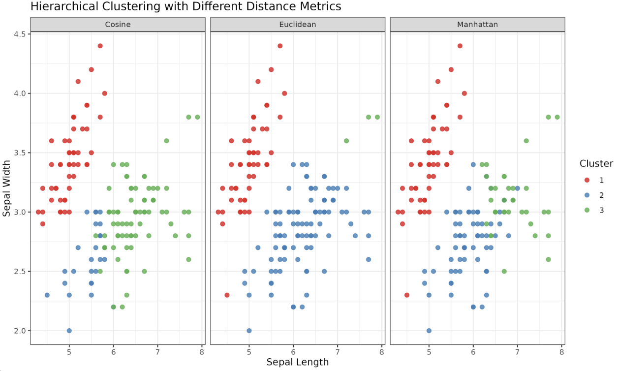
Let’s visualize how the choice of distance metric affects clustering. Prepare Data for Plotting: R library(ggplot2) library(dplyr) library(tidyr) plot_data <- as.data.frame(dataset) plot_data$Sepal.Length <- iris$Sepal.Length plot_data$Sepal.Width <- iris$Sepal.Width plot_data$Euclidean <- as.factor(labels_euc) plot_data$Manhattan <- as.factor(labels_man) plot_data$Cosine <- as.factor(labels_cos) plot_data_long <- plot_data %>% select(Sepal.Length, Sepal.Width, Euclidean, Manhattan, Cosine) %>% pivot_longer(cols = c(Euclidean, Manhattan, Cosine), names_to = "Metric", values_to = "Cluster") Plot with ggplot2: R ggplot(plot_data_long, aes(x = Sepal.Length, y = Sepal.Width, color = Cluster)) + geom_point(size = 2, alpha = 0.8) + facet_wrap(~ Metric, nrow = 1) + labs(title = "Hierarchical Clustering with Different Distance Metrics", x = "Sepal Length", y = "Sepal Width") + theme_bw() + scale_color_brewer(palette = "Set1")

Using R's hclust and dist with Different Metrics

You can also use R’s built-in functions for hierarchical clustering with different distance metrics. Euclidean and Manhattan: Rd_euc <- dist(dataset, method = "euclidean") hc_euc <- hclust(d_euc, method = "average") labels_euc <- cutree(hc_euc, k = n_clusters) d_man <- dist(dataset, method = "manhattan") hc_man <- hclust(d_man, method = "average") labels_man <- cutree(hc_man, k = n_clusters)d_euc <- dist(dataset, method = "euclidean") hc_euc <- hclust(d_euc, method = "average") labels_euc <- cutree(hc_euc, k = n_clusters) d_man <- dist(dataset, method = "manhattan") hc_man <- hclust(d_man, method = "average") labels_man <- cutree(hc_man, k = n_clusters) Cosine Distance (Manual Calculation): 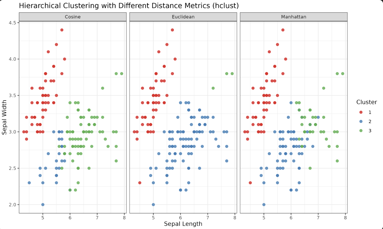Rcosine_distance_matrix <- function(X) { n <- nrow(X) dist_mat <- matrix(0, n, n) for (i in 1:(n-1)) { for (j in (i+1):n) { sim <- sum(X[i, ] * X[j, ]) / (sqrt(sum(X[i, ]^2)) * sqrt(sum(X[j, ]^2))) dist <- 1 - sim dist_mat[i, j] <- dist dist_mat[j, i] <- dist } } as.dist(dist_mat) } d_cos <- cosine_distance_matrix(dataset) hc_cos <- hclust(d_cos, method = "average") labels_cos <- cutree(hc_cos, k = n_clusters)cosine_distance_matrix <- function(X) { n <- nrow(X) dist_mat <- matrix(0, n, n) for (i in 1:(n-1)) { for (j in (i+1):n) { sim <- sum(X[i, ] * X[j, ]) / (sqrt(sum(X[i, ]^2)) * sqrt(sum(X[j, ]^2))) dist <- 1 - sim dist_mat[i, j] <- dist dist_mat[j, i] <- dist } } as.dist(dist_mat) } d_cos <- cosine_distance_matrix(dataset) hc_cos <- hclust(d_cos, method = "average") labels_cos <- cutree(hc_cos, k = n_clusters)

Visualizing hclust Results

Prepare Data: R plot_data$Euclidean <- as.factor(labels_euc) plot_data$Manhattan <- as.factor(labels_man) plot_data$Cosine <- as.factor(labels_cos) plot_data_long <- plot_data %>% select(Sepal.Length, Sepal.Width, Euclidean, Manhattan, Cosine) %>% pivot_longer(cols = c(Euclidean, Manhattan, Cosine), names_to = "Metric", values_to = "Cluster") plot_data$Euclidean <- as.factor(labels_euc) plot_data$Manhattan <- as.factor(labels_man) plot_data$Cosine <- as.factor(labels_cos) plot_data_long <- plot_data %>% select(Sepal.Length, Sepal.Width, Euclidean, Manhattan, Cosine) %>% pivot_longer(cols = c(Euclidean, Manhattan, Cosine), names_to = "Metric", values_to = "Cluster") Plot: R ggplot(plot_data_long, aes(x = Sepal.Length, y = Sepal.Width, color = Cluster)) + geom_point(size = 2, alpha = 0.8) + facet_wrap(~ Metric, nrow = 1) + labs(title = "Hierarchical Clustering with Different Distance Metrics (hclust)", x = "Sepal Length", y = "Sepal Width") + theme_minimal() + scale_color_brewer(palette = "Set1") ggplot(plot_data_long, aes(x = Sepal.Length, y = Sepal.Width, color = Cluster)) + geom_point(size = 2, alpha = 0.8) + facet_wrap(~ Metric, nrow = 1) + labs(title = "Hierarchical Clustering with Different Distance Metrics (hclust)", x = "Sepal Length", y = "Sepal Width") + theme_minimal() + scale_color_brewer(palette = "Set1")

Key Takeaways

Distance metrics define how similarity is measured in clustering. Euclidean, Manhattan, and Cosine distances each have unique properties and applications. The choice of metric can significantly change clustering results, as seen in the visualizations.

Lesson Summary and Practice

Excellent work! You've just mastered the concepts and the importance of distance metrics in hierarchical clustering. You've implemented these metrics in R and applied them in the agglomerative clustering algorithm. In the end, you studied the impact of these distance metrics on the clustering results using ggplot2 for clear and effective visualization. Next, get ready to solidify this knowledge through related exercises!