Hierarchical Clustering is a crucial part of unsupervised machine learning. It is a powerful tool for grouping data based on inherent patterns and shared characteristics. By visually representing the hierarchy of clusters, it provides deep insights into the intricacies and overlapping structures of our data.

Hierarchical Clustering operates broadly through two approaches — Agglomerative and Divisive. The Agglomerative technique, also known as 'bottom-up,' begins by treating every data point as a distinct cluster and then merges them until only one cluster remains. Conversely, the Divisive methodology, termed 'top-down,' begins with all data points in a single cluster and splits them progressively until each point forms its own cluster.

One of the most common forms of Hierarchical Clustering is Agglomerative Hierarchical Clustering. It starts with every single object in a single cluster. Then, in each successive iteration, it merges the closest pair of clusters and updates the similarity (or distance) between the newly formed cluster and each old cluster. The algorithm repeats this process until all objects are in a single remaining cluster.

The Agglomerative Hierarchical Clustering involves the following major steps:

• Compute the similarity (or distance) matrix containing the distance between each pair of objects in the dataset.
• Represent each data object as a singleton cluster.
• Repeat merging the two closest clusters and updating the distance matrix until only one cluster remains.
• The output is a tree-like diagram named dendrogram which represents the order and distances (similarity) of merges during the algorithm execution.

The Distance Matrix is a foundational element in hierarchical clustering that plays a critical role in understanding the relations and proximities between data points. Essentially, it is a square matrix where each element (i, j) represents the distance between the i-th and the j-th points in the dataset. The choice of distance metric (Euclidean, Manhattan, Cosine, etc.) can significantly influence the clustering outcome and is crucial to the coherence of the resulting clusters.

Distance matrix representation in linear algebra is as follows:

1. Initial Cluster Formation: It provides the initial groundwork for forming clusters by quantifying the closeness or similarity between individual data points or clusters.

2. Cluster Merging Strategy: It is essential to decide which clusters to merge at each step of the agglomerative clustering process. Clusters with the smallest distances between them are merged, promoting more natural groupings in the data.

3. Efficiency in Recalculation: After merging clusters, updating the distance matrix (instead of recalculating all distances from scratch) speeds up the clustering process considerably. Different linkage criteria (single, complete, average, etc.) provide various strategies for updating these distances.

4. Visual Representation and Analysis: The final dendrogram, which visualizes the process of hierarchical clustering, is fundamentally reliant on the distances computed and stored in this matrix. This visualization aids in determining the appropriate number of clusters by identifying significant gaps in the distances at which clusters merge.

Understanding and appropriately calculating the distance matrix is, therefore, a precursor to effectively implementing hierarchical clustering algorithms and extracting meaningful insights from complex datasets.

We'll use the Iris dataset and some standard R libraries — ggplot2 for data visualization.

We plot our dataset with GGally's ggpairs, which aids in drawing more attractive and informative statistical graphics:

Output plot:

Step 1: Euclidean Distance Function

Let's define a function to calculate the Euclidean distance between two points:

Now we can define a function that computes the distance matrix between clusters (using average linkage):

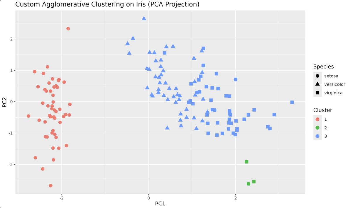
Now, let's define the main function for Agglomerative Clustering:

Let's visualize the clustering using the first two principal components for better separation:

Output plot:

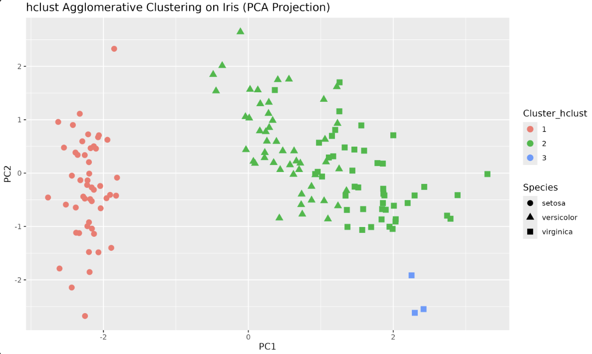
R provides an optimized, efficient implementation of Hierarchical Clustering through the hclust() function. Let's try it with our Iris dataset.

Step 1: Compute Distance Matrix

Step 2: Perform Hierarchical Clustering

Step 3: Cut Tree into Clusters

Step 4: Visualize the Clusters

Output plot:

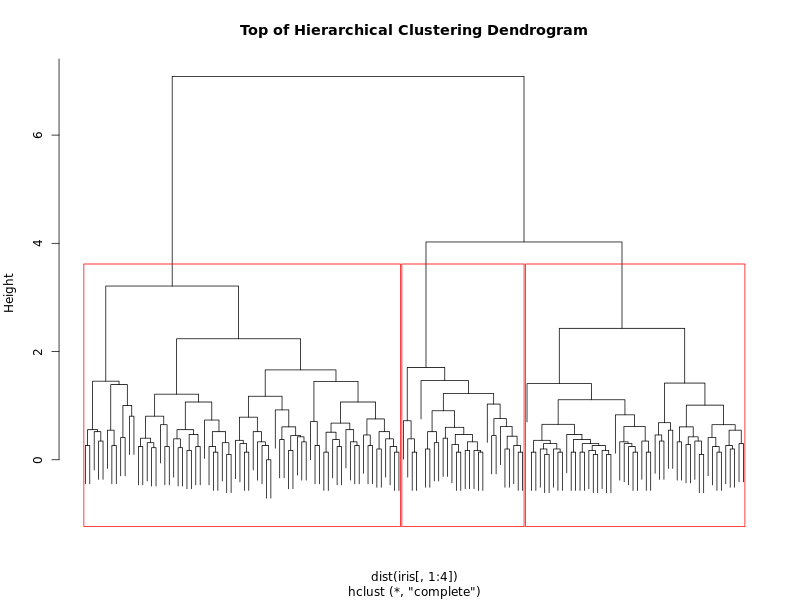
Here, we are plotting the dendrogram produced by hierarchical clustering on the Iris dataset (using only the four numeric features). The dendrogram visually represents how clusters are formed at each step of the agglomerative process.

Output:

Congratulations! You've successfully broken down the nuances of Hierarchical Clustering, focusing on Agglomerative Clustering, and brought Hierarchical Clustering to life using R. You implemented the algorithm from scratch, visualized the results with ggplot2, and compared your results to R's built-in hclust function. Practice tasks await next, offering the perfect platform to apply acquired concepts and deepen your understanding of Hierarchical Clustering. Carry this momentum forward, and let's forge ahead into the captivating world of Hierarchical Clustering!