In the previous lesson, you successfully connected Grafana to your PostgreSQL database and verified that the connection was working. That was an important first step, but now comes the exciting part — actually using that connection to create visualizations. In this lesson, you'll move from simply being connected to actively querying your data and seeing it displayed on a chart.

You might be thinking, "I know SQL, so writing queries in Grafana should be straightforward, right?" Well, almost. Grafana does use SQL, but it adds some special functionality on top of it. When you write a query for a Grafana panel, you're not just retrieving data — you're retrieving data in a specific format that Grafana can transform into beautiful, interactive charts. Think of it as SQL with superpowers that connect directly to Grafana's time range controls and visualization engine.

By the end of this lesson, you'll have written your first time-series query that displays CPU usage across different hosts. You'll understand the specific structure Grafana needs and learn to use special macros that make your queries work seamlessly with Grafana's interface. This pattern you learn here will become the foundation for every time-series panel you create going forward.

Note: From this unit forward, anonymous mode is enabled in all practice exercises so you won't need to sign in each time. This is for lab convenience only—never use anonymous access in production. In real environments, always require proper authentication and restrict permissions according to best practices. For more information, see the Grafana authentication documentation.

Before you can write any queries, you need to know where to write them. Grafana provides a dedicated space called the Explore section specifically for testing and developing queries before adding them to dashboards. You can find Explore in the left sidebar — it looks like a compass icon. When you click on it, Grafana opens a query workspace where you can experiment with data retrieval and visualization.

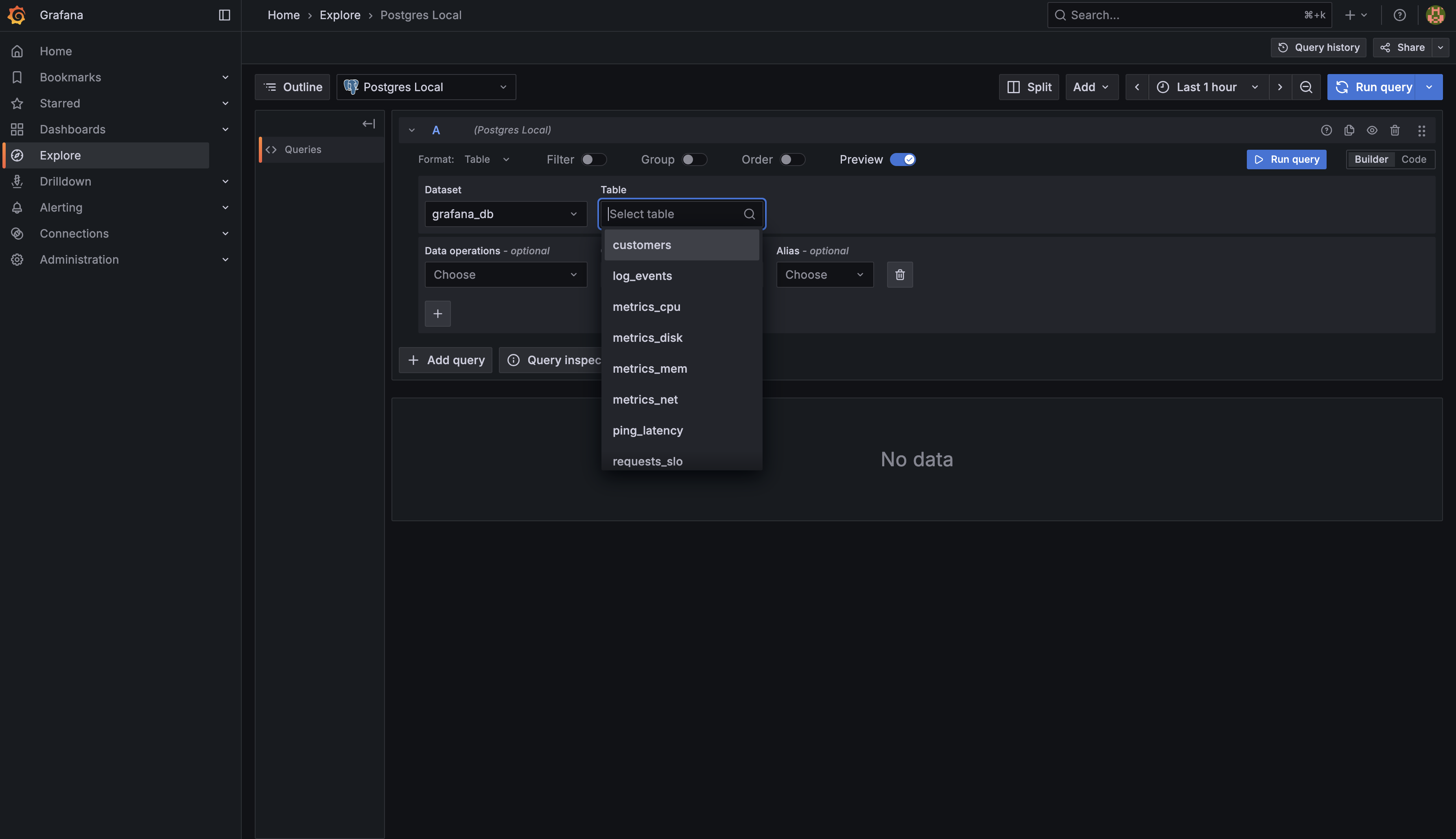
Once you're in Explore, notice that your configured Postgres data source — in this lab environment, it's named Postgres Local — is already selected at the top. When you open Explore with this data source, Grafana helpfully displays a list of available tables in your database. You can see tables like log_events, metrics_cpu, metrics_disk, and others that contain your demo metrics data. This gives you a quick reference of what data is available to query.

What you're looking at right now is the Builder tab — Grafana's visual, form-based interface for constructing queries. You can select tables and columns from dropdowns and build queries without writing SQL directly. While the Builder can be useful for simple queries, we're going to work with the Code tab instead, which gives you much more freedom and control.

Click on the Code tab. This is where you can write raw SQL queries with complete flexibility. Let's verify that we can access the same table information programmatically. In the code editor, enter the following query:

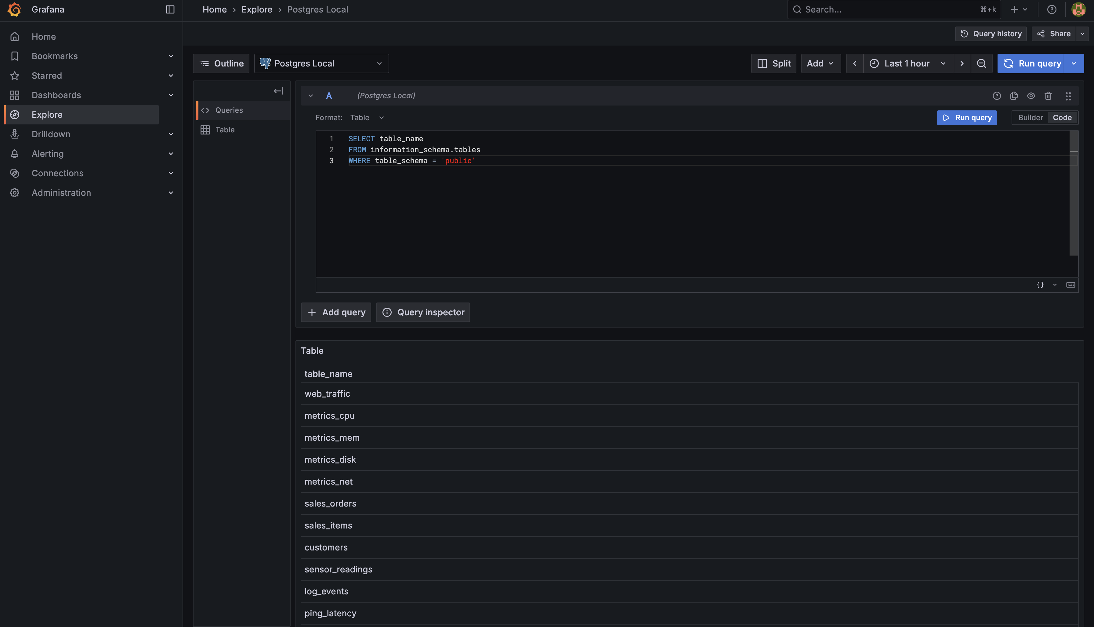
Now click the Run Query button in the upper right corner of the query editor. When you execute this query, you'll see the same list of tables in the results panel below — log_events, metrics_cpu, metrics_disk, and all the other tables that were shown in the Builder tab's sidebar. This confirms that you have full access to query the database structure and data.

The Code tab interface has several components: the text area where you write your SQL query, the Run Query button to execute it, formatting options at the top, and a results panel at the bottom where you'll see both the data returned and a preview visualization. The interface might look a bit different from a standard SQL client you may have used before, but the core concept is the same — you write a query, execute it, and see results. For this course, we'll be working exclusively with the Code tab, as it gives you the power to write exactly the queries you need for time-series visualization.

Now that you know how to navigate the query editor, let's take a closer look at the data you'll be working with. Among all those tables in your database, metrics_cpu is going to be your best friend for this lesson. Think of it as a logbook that records how hard each of your servers is working at any given moment.

The metrics_cpu table is beautifully simple — it has just three columns:

• ts — Short for "timestamp," this records exactly when each CPU measurement was taken
• host — This identifies which server the measurement came from (like "host-a", "host-b", etc.)
• usage — This is the actual CPU usage percentage at that moment

Let's peek at what this data actually looks like. Run this quick query:

You'll see results similar to this:

Notice the pattern? Every minute (check those timestamps!), the system records CPU usage for each host. At 18:48:04, host-a was running at 28% CPU while host-b was cruising at 24.9%. A minute later, both hosts' usage changed. This is time-series data in its purest form — measurements taken at regular intervals over time.

This simple structure is actually perfect for what we're about to do. You have timestamps (when), identifiers (which server), and measurements (how much CPU). That's everything you need to create compelling visualizations that show trends, spikes, and patterns over time.

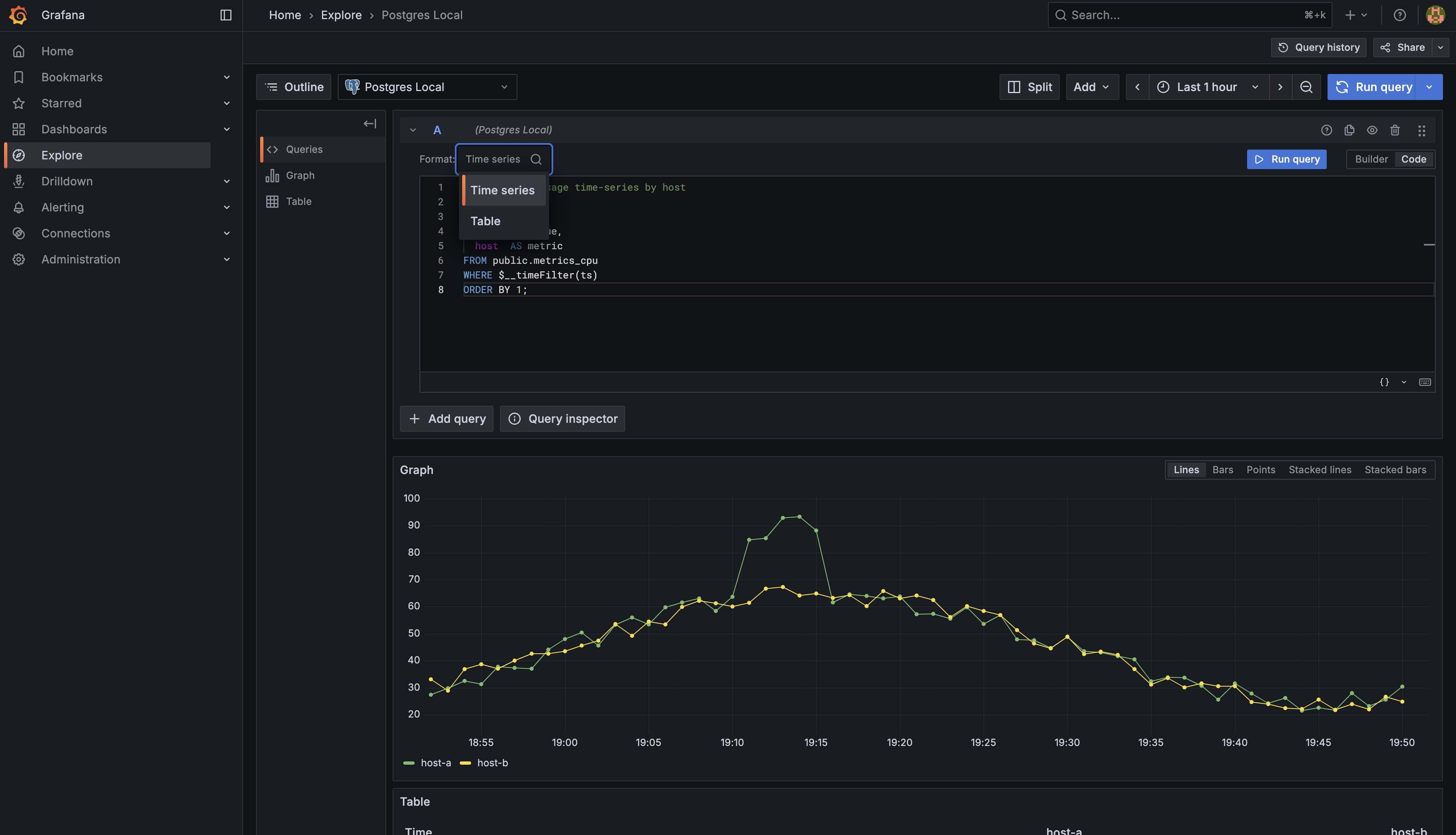
Now here's where things get interesting. You've got this perfectly good table with your data, but Grafana wants it served in a specific way. When you're building a time-series panel, Grafana expects your query to return exactly three columns with precise names: time, value, and metric.

Wait a minute — didn't we just say metrics_cpu has columns named ts, usage, and host? Exactly! This is where SQL's renaming capabilities come to the rescue. You're going to transform your table's column names into what Grafana expects. Think of it as translating from one language to another:

• Your ts column becomes time — the when
• Your usage column becomes value — the measurement
• Your host column becomes metric — the identifier

Note: If your table has more than 3 columns, you only need to select and alias the 3 columns Grafana expects for this pattern: time, value, and metric. You can ignore extra columns in your SELECT statement.

Here's the beautiful part: when you rename host to , Grafana automatically knows to draw a separate line for each unique host value. If you have data from three servers, you'll get three colored lines on your chart. If you have ten servers, you'll get ten lines. Grafana reads the column and thinks, "Ah, I need to group these data points and visualize them separately." No extra configuration needed!

Now, here's where things get interesting. Instead of writing long, complicated SQL date formatting functions, Grafana gives you special shortcuts called macros. They're like having a helpful assistant who writes the boring SQL for you.

The first macro you'll love is $__time(ts). When you use this in your query, you're basically saying: "Hey Grafana, take this timestamp column called ts and format it exactly how you need it for visualization." Grafana handles all the technical details behind the scenes. No need to remember database-specific date functions — the macro does it for you.

The second macro is even cooler: $__timeFilter(ts). This one is pure magic. You know that time range picker at the top of Grafana dashboards where you can select "Last 15 minutes" or "Last 7 days"? Well, $__timeFilter(ts) automatically connects your query to that picker.

Let's say someone selects "Last 24 hours" in the dashboard. Your query instantly filters to show only the last 24 hours of data. They change it to "Last week"? Your query automatically adjusts. You don't have to write different queries for different time ranges — the macro handles everything. It's like having a query that reads the user's mind!

These macros are what transform your basic SQL into a dynamic, interactive Grafana experience. Once you get comfortable with them, you'll wonder how you ever lived without them.

Here's an important detail: technically, the time picker will still work even if you don't use $__timeFilter() — Grafana will filter the data on its end. But here's the catch: without the macro, your database loads every single row from the table and sends all that data to Grafana, which then throws away everything outside your selected time range. With small demo datasets, you won't notice. But in production with millions of rows? Your query will crawl to a halt. The $__timeFilter() macro is what tells PostgreSQL "only send data from the selected time period," making your database do the heavy lifting efficiently with indexes. Always use it — it's the difference between a query that takes 10 seconds versus one that takes 10 milliseconds.

Let's now put all the pieces together and build your first Grafana time-series query. You understand your source data (metrics_cpu with its ts, host, and usage columns), you know what Grafana expects (columns named time, metric, and value), and you've learned about the magical macros. Time to combine them!

Start with the SELECT clause. You need to transform your three source columns into Grafana's expected format. For the time column, use $__time(ts) — this macro automatically formats your timestamp. For the value column, select usage AS value to rename your CPU percentage. For the metric column, select host AS metric to identify which server each measurement belongs to.

The FROM clause is straightforward: FROM public.metrics_cpu tells the database where to get the data.

Your WHERE clause is where the second macro shines. Add WHERE $__timeFilter(ts) to connect your query to Grafana's time range picker. This single line makes your query dynamically responsive to user selections.

Finally, add ORDER BY 1 to sort results by the first column (time) in chronological order. This ensures your visualization displays data points from oldest to newest.

Here's the complete query:

Congratulations! You've just learned the fundamental pattern for building time-series panels in Grafana: select your timestamp with $__time(), alias your measurement as value, alias your identifier as metric, add $__timeFilter() to connect to the time picker, and order chronologically. That's it! This same pattern works for CPU, memory, disk, network — any metric with timestamps.

In the upcoming practice exercises, you'll build this query from scratch. You'll start by discovering available tables, then construct the CPU query step by step. Don't be afraid to experiment and modify the queries to see what happens. The best way to learn Grafana is by doing. Let's get started with practice!