In the previous lesson, you successfully rendered your first 3D object — a sphere — using ray tracing. However, if you look closely at the result, you'll notice something that might seem a bit disappointing: the sphere appears as a flat red circle. There's no sense of depth, no curvature, no indication that you're looking at a three-dimensional object rather than a simple 2D disk painted on the screen.

This flatness occurs because you're coloring every pixel that hits the sphere with the exact same solid red color, regardless of where on the sphere's surface that ray intersects. In the real world, objects appear three-dimensional because light interacts differently with different parts of their surfaces depending on the surface orientation. A sphere's surface curves away from us, and this curvature should be visible in how it's shaded.

In this lesson, you'll learn how to give your sphere a sense of depth and dimensionality by using surface normals. By the end of this lesson, your flat red circle will transform into a sphere that clearly looks three-dimensional, with color gradients that reveal its curved surface. You'll accomplish this by computing the surface normal at each intersection point and mapping that normal vector directly to RGB color values. While this isn't yet realistic lighting (that comes later), it's a crucial stepping stone that will help you understand how surface orientation affects appearance and prepare you for implementing proper lighting models.

The mathematics involved are straightforward, and you'll see that with just a few modifications to your existing code, you can achieve dramatically more convincing results. Let's begin by understanding what surface normals are and why they're so important in computer graphics.

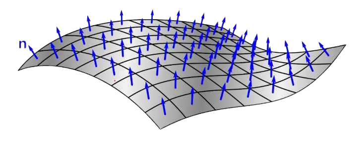
A surface normal is a vector that points perpendicular to a surface at a specific point. Think of it as an arrow sticking straight out from the surface, indicating which direction the surface is "facing" at that location. Surface normals are fundamental in computer graphics because they encode information about surface orientation, which is essential for calculating how light should interact with that surface.

For a sphere, the surface normal at any point has a particularly elegant property: it always points directly outward from the sphere's center, passing through the surface point. This makes intuitive sense — if you imagine standing on the surface of a perfectly round ball, "straight up" from your perspective would be the direction pointing away from the ball's center through where you're standing.

Mathematically, if we have a sphere centered at point c and a point p on the sphere's surface, the outward normal at p is simply the vector from c to p, normalized to unit length. We can write this as: N = (p - c) / r, where r is the sphere's radius. Since p is on the sphere's surface, the distance from c to p is exactly r, so dividing by r gives us a unit vector (a vector with length 1). In our code, we'll use the unit_vector() function to achieve the same result: unit_vector(p - center).

Why do we care about unit length? In computer graphics, normals are conventionally kept at unit length for consistency and to simplify calculations. When we later implement lighting models, having unit-length normals means we can use them directly in dot products without worrying about scaling factors. For now, unit-length normals also ensure that our color mapping (which we'll discuss shortly) produces consistent results regardless of the sphere's size.

Our current hit_sphere() function has a limitation that prevents us from easily computing surface normals. As you'll recall from the previous lesson, the function returns a single double value: the parameter t where the ray hits the sphere, or -1.0 if there's no hit. This works fine for simply detecting whether a hit occurred, but to compute the surface normal, we need to know the exact value of t so we can calculate the hit point using r.at(t).

The problem is that once hit_sphere() returns, we've lost access to that t value in our ray_color() function. We could call hit_sphere() twice — once to check if there's a hit, and again to get the t value — but that would be inefficient and inelegant. Instead, we'll use a common pattern in C++ programming: we'll change the function to return a bool indicating whether a hit occurred, and pass the t value back through a reference parameter.

A reference parameter allows a function to modify a variable that belongs to the caller. When we declare a parameter with an ampersand (&), like double& t_hit, we're saying that instead of receiving a copy of the value, the function receives a reference to the original variable. Any changes the function makes to will be reflected in the caller's variable. This pattern is extremely common in ray tracing code because intersection functions often need to return multiple pieces of information: whether a hit occurred, where it occurred, and potentially other data like the surface normal or material properties.

Now that our hit_sphere() function can tell us both whether a hit occurred and where it occurred (via the t value), we can compute the actual 3D point where the ray intersected the sphere's surface. This hit point is essential because it's what we need to calculate the surface normal.

Computing the hit point is straightforward using our ray's at() method. Remember that a ray is defined parametrically as r(t) = o + td, where o is the origin and d is the direction. Our ray class provides the at(t) method that implements exactly this calculation. So if hit_sphere() tells us that the ray hits the sphere at parameter value t, we can find the hit point with point3 p = r.at(t).

Once we have the hit point, calculating the outward surface normal is equally simple. As we discussed earlier, for a sphere centered at c, the normal at point p is the unit vector pointing from c to p. In code, this becomes vec3 N = unit_vector(p - center). The subtraction p - center gives us a vector pointing from the sphere's center to the hit point, and unit_vector() normalizes it to length 1.

Why do we use unit_vector() here? While we could work with the unnormalized vector , keeping normals at unit length is a standard convention in computer graphics. Unit-length normals simplify many calculations, particularly when we implement lighting models in future lessons. For our current purpose of visualizing normals as colors, using unit vectors ensures that the color mapping we're about to implement produces consistent, predictable results. A unit vector's components always range from -1 to 1, which makes the transformation to RGB values straightforward.

Now comes the interesting part: how do we visualize these surface normals? The technique we'll use is to map the normal vector's components directly to RGB color values. This creates a color-coded visualization where different surface orientations produce different colors, immediately revealing the sphere's three-dimensional structure.

The challenge is that normal vector components range from -1 to 1 (since we're using unit vectors), but RGB color channels need values in the range 0 to 1 (which our write_color() function then scales to 0-255 for the PPM format). We need a transformation that maps the range [-1, 1] to [0, 1]. The mathematical transformation we'll use is: color_component = 0.5 * (normal_component + 1). Let's understand why this works. Adding 1 to a value in the range [-1, 1] gives us a value in the range [0, 2]. Multiplying by 0.5 then scales this to [0, 1], which is exactly what we need.

We apply this transformation to all three components of the normal vector simultaneously. If our normal is N = (Nx, Ny, Nz), our color becomes: color = 0.5 * (N + 1) = 0.5 * (Nx + 1, Ny + 1, Nz + 1). In our code, we can write this concisely as 0.5*color(N.x()+1, N.y()+1, N.z()+1), where we're using our color type (which is just a vec3) and taking advantage of scalar multiplication.

What does this mapping mean visually? The X component of the normal maps to the red channel, the Y component to green, and the Z component to blue. Consider what this means for different points on the sphere. At the rightmost visible point of the sphere, the normal points in the positive X direction, so Nx is close to 1, giving us a strong red component. At the topmost point, the normal points in the positive Y direction, producing a strong green component. At the point closest to the camera, the normal points in the positive Z direction (toward us), creating a strong blue component.

Points where the normal has negative components will have reduced color intensity in the corresponding channels. For example, at the leftmost visible point, Nx is close to -1, which maps to a red value near 0 (dark). The result is a sphere with a beautiful gradient of colors that clearly shows how the surface curves in three-dimensional space. The center of the sphere (the point facing directly toward the camera) will appear bluish because the Z component dominates, while the edges will show reds, greens, and various combinations depending on their orientation.

Let's now put all the pieces together and see the complete updated code. Here's the full ray_color() function with our normal-based shading:

Let's walk through the complete flow from ray to colored pixel. For each pixel in our image, we construct a ray from the camera through that pixel. We then call ray_color() with this ray. Inside ray_color(), we first attempt to intersect the ray with our sphere by calling hit_sphere(). We pass a reference to the variable t, which will receive the intersection distance if a hit occurs.

If hit_sphere() returns true, we know the ray hit the sphere, and t contains the distance to the hit point. We compute the actual 3D hit point using r.at(t), which evaluates the ray equation at parameter t. With the hit point in hand, we calculate the outward surface normal by subtracting the sphere's center from the hit point and normalizing the result. This normal vector tells us which direction the sphere's surface is facing at this particular intersection point.

We then transform this normal into a color by applying our mapping formula: we add 1 to each component (shifting the range from [-1,1] to [0,2]) and multiply by 0.5 (scaling to [0,1]). This gives us an RGB color where the red channel represents the X component of the normal, green represents Y, and blue represents Z. We return this color, which will be written to the corresponding pixel in our output image.

When you examine your rendered image, take a moment to really look at the colors and understand what they're telling you about the sphere's geometry. The center of the sphere, where the surface faces directly toward the camera, should appear predominantly blue or cyan. This makes sense because at that point, the surface normal points in the positive Z direction (toward you), and the Z component maps to the blue channel.

As you move toward the edges of the sphere, you'll see the colors shift. The right edge will show more red because the normals there point in the positive X direction. The top edge will show more green because those normals point in the positive Y direction. The left and bottom edges will be darker because the normals there have negative X and Y components, respectively, which map to lower color values. The smooth gradients between these regions reveal how the sphere's surface continuously curves in three-dimensional space.

This color-coded visualization of normals is doing something profound: it's showing you the orientation of the surface at every visible point. Even though we haven't implemented any actual lighting yet, the varying colors create a strong sense of depth and three-dimensionality. Your brain interprets these color gradients as evidence of a curved surface, even though you know intellectually that you're just looking at a flat image on a screen.

What you've accomplished in this lesson is a crucial stepping stone toward realistic rendering. Surface normals are the foundation of almost all lighting calculations in computer graphics. In upcoming lessons, when we implement proper lighting models like diffuse and specular reflection, we'll use these same normal vectors to calculate how light bounces off the surface. The Phong reflection model, for instance, uses the angle between the surface normal and the light direction to determine how bright a surface appears. By learning to compute and visualize normals now, you're preparing yourself for these more advanced techniques.

In the practice exercises that follow, you'll get hands-on experience experimenting with this normal-based shading. You'll try positioning spheres at different locations, observe how the colors change based on the sphere's position relative to the camera, and explore what happens when you modify the normal calculation. These exercises will deepen your intuition about how surface orientation affects appearance and prepare you for the next major step in your ray tracing journey: implementing realistic lighting that will make your scenes truly come alive.