In the previous lesson, you wrote your first C++ program that printed "Hello, Raytracer!" to the terminal. That simple program established the basic structure we'll use throughout this course and verified that your development environment works correctly. Now we're ready to take an exciting leap forward: instead of outputting text, we're going to generate actual visual images.

This transition from text to images is a pivotal moment in your ray tracing journey. Every ray tracer, no matter how sophisticated, ultimately does one thing: it produces image data. The stunning photorealistic renders you see in movies, the beautiful architectural visualizations, and the realistic reflections in modern games — they all start with the same fundamental task we're about to tackle: writing color values for each pixel in an image.

In this lesson, you'll learn how to represent images as grids of colored pixels and how to output them in a format called PPM (Portable Pixmap). We'll start with something deliberately simple: a solid red image. This might seem basic compared to the complex 3D scenes we'll eventually render, but it establishes the foundation for everything to come. Once you understand how to generate and output image data, adding ray tracing to calculate what colors those pixels should be becomes a natural next step.

By the end of this lesson, you'll have a program that generates a complete image file. You'll see your code produce visual output for the first time, and you'll understand the structure that every image-generating program follows. This is where your ray tracer truly begins.

Before we can generate images, we need to understand what images actually are at a fundamental level. When you look at a photograph on your screen or a frame from a movie, you're seeing a grid of tiny colored dots called pixels. The word "pixel" is short for "picture element," and it represents the smallest unit of an image that we can control individually.

Think of an image like a mosaic made of tiny colored tiles. Each tile is a single color, and when you step back and look at all the tiles together, they form a complete picture. Pixels work the same way. A typical image might be 1920 pixels wide and 1080 pixels tall, giving us over two million individual pixels. Each one contributes its small part to the overall image.

Every pixel has a color, and in computer graphics, we typically represent colors using the RGB color model. RGB stands for Red, Green, and Blue — the three primary colors of light. This might seem different from what you learned in art class, where the primary colors are red, yellow, and blue. That's because mixing paint (subtractive color) works differently from mixing light (additive color). When you combine red, green, and blue light in different proportions, you can create any color visible to the human eye.

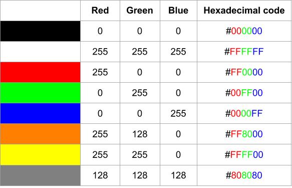
Each color component in RGB has an intensity value that tells us how much of that color to include. In most image formats, including the one we'll use today, these intensity values range from 0 to 255. A value of 0 means none of that color, while 255 means the maximum amount. For example, pure red would be represented as red=255, green=0, blue=0. Pure white, which is all colors at maximum intensity, would be red=255, green=255, blue=255. Black, the absence of light, would be red=0, green=0, blue=0.

Now that we understand what pixels are, we need a way to save them to a file that image viewers can display. There are many image formats you've probably heard of: JPEG, PNG, GIF, and others. These formats are sophisticated and use compression to make files smaller, but that complexity makes them challenging to work with when you're learning. Instead, we're going to use a format called PPM, which stands for Portable Pixmap.

PPM is perfect for learning because it's incredibly simple and human-readable. Unlike formats like PNG that store data in compressed binary form, PPM files are plain text. You can open a PPM file in any text editor and see exactly what's inside. This transparency makes it easy to understand what your program is doing and to debug problems when they arise.

A PPM file has a straightforward structure with four main parts. First comes the magic number, which is just a special code that identifies what type of file this is. For ASCII-based PPM files (the kind we'll create), the magic number is P3. This tells image viewers, "Hey, I'm a PPM file with text-based pixel data."

Next come the image dimensions: the width and height in pixels. These are just two numbers separated by a space. For example, 256 256 means the image is 256 pixels wide and 256 pixels tall.

The third part is the maximum color value. This tells the image viewer what range the color values use. We'll always use 255, which means our color components range from 0 to 255 as we discussed earlier.

Finally comes the actual pixel data: the RGB values for every pixel in the image. These are written as triplets of numbers, with each triplet representing one pixel's red, green, and blue components.

Let's look at a tiny example to make this concrete. Here's a complete PPM file for a 3×2 image (six pixels):

Let's break this down line by line. The first line, P3, is our magic number identifying this as an ASCII PPM file. The next line starting with # is a comment, which are allowed in PPM files and help explain the structure. The line tells us this image is 3 pixels wide and 2 pixels tall. The next line, , sets our maximum color value. Then comes the pixel data.

Now let's start building our image generator. We'll begin with the PPM header, which contains the metadata about our image. Remember from the previous section that the header consists of three parts: the magic number, the dimensions, and the maximum color value.

Here's how we write the header in C++:

Let's examine this code carefully. At the top, we include <iostream> just like in our "Hello, Raytracer!" program. This gives us access to std::cout, which we'll use to output our image data.

Inside main(), we first define two constants: image_width and image_height. We're using the const keyword because these values won't change during our program's execution. We've chosen 256 for both dimensions, which will give us a square image with 65,536 pixels. The number 256 is convenient because it's a power of 2, which computers handle efficiently, and it's large enough to see detail but small enough to generate quickly.

The next line is where we output the PPM header. Let's break down this statement: std::cout << "P3\n" << image_width << ' ' << image_height << "\n255\n";. We're using std::cout with the << operator multiple times in sequence. Each << sends something to the output stream.

Now that we have our header, we need to generate the actual pixel data. Remember, our image is 256 pixels wide and 256 pixels tall, which means we need to output 65,536 RGB triplets. Writing these by hand would be impossible, so we'll use loops to generate them systematically.

The structure we need is a nested loop: an outer loop that iterates through each row of the image, and an inner loop that iterates through each pixel in that row. Here's the complete code with the pixel generation added:

Let's examine the loop structure carefully. The outer loop uses the variable j to represent the row number. Notice something interesting: we start at image_height - 1 (which is 255) and count down to 0. This might seem backward, but there's a good reason for it.

In many graphics systems, including the one we're building, we think of the coordinate system with the origin (0, 0) at the bottom-left corner of the image. The y-coordinate increases as we move up. However, when we write pixel data to a PPM file, we write it from top to bottom. By starting our loop at the highest row number and counting down, we're writing the top row of the image first, then working our way down. This ensures that when an image viewer displays our PPM file, it appears right-side up.

The loop condition j >= 0 means we continue as long as j is greater than or equal to zero. The update expression decrements by one after each iteration. So our outer loop runs 256 times, once for each row.

When you run the program we've built so far, it generates the image data very quickly. But as we add more complex ray tracing calculations in future lessons, rendering an image might take seconds, minutes, or even longer. It's helpful to have feedback about how the rendering is progressing so you know the program is working and haven't accidentally created an infinite loop.

We'll add progress feedback that displays which row we're currently rendering. Here's the updated code:

Notice we've added two new lines. At the beginning of the outer loop, we have: std::cerr << "\rScanlines remaining: " << j << ' ' << std::flush;. And after the loops complete, we have: std::cerr << "\nDone. \n";.

Let's understand what's happening here. First, notice we're using std::cerr instead of std::cout. Both are output streams, but they serve different purposes. std::cout is the standard output stream, which we use for the actual program output — in our case, the image data. std::cerr is the standard error stream, which is typically used for diagnostic messages, warnings, and errors.

Why does this distinction matter? When we run our program, we'll redirect the standard output to a file to save our image. If we used std::cout for our progress messages, those messages would end up in the image file and corrupt it. By using , we ensure our progress messages go to the terminal where we can see them, while our image data goes to the file where it belongs.

Now that we have a complete program, let's talk about how to run it and view the resulting image. The key concept here is output redirection, which is a feature of command-line shells that lets you send a program's output to a file instead of displaying it on the screen.

When you run a program normally, its output appears in your terminal. But we want to save our image data to a file so we can view it with an image viewer. On most systems, you would do this by running your program with output redirection like this:

The > symbol tells the shell to redirect the standard output (everything sent to std::cout) to a file named image.ppm. The progress messages we send to std::cerr still appear in the terminal because we're only redirecting standard output, not standard error.

On this platform, the environment handles this process for you automatically. When you run your code, the system captures the output, saves it as an image file, and displays it in the interface. You don't need to worry about redirection commands or file management — you can focus entirely on writing the code that generates the image.

When you run the complete program we've built in this lesson, you'll see a solid red square. Every pixel in the 256×256 image will be pure red (RGB: 255, 0, 0). This might not seem impressive compared to the complex scenes we'll eventually render, but it represents a major milestone. You've successfully generated image data, formatted it correctly as PPM, and produced a viewable image file.

If you were to open the PPM file in a text editor (which you can do on your own computer, though it's not necessary on CodeSignal), you'd see the header followed by 65,536 lines of 255 0 0. The file would be quite large — around 500 kilobytes — because we're storing everything as text. This is one reason why compressed image formats exist, but for our purposes, the simplicity of PPM is worth the extra file size.

The important thing to understand is the flow: your program generates RGB values for each pixel, outputs them in PPM format to standard output, that output gets saved to a file, and an image viewer interprets the PPM format to display the colored pixels. This same flow will apply to every image we generate throughout this course. The only thing that will change is how we calculate those RGB values — instead of hardcoding them to red, we'll use ray tracing to determine what color each pixel should be based on the 3D scene we're rendering.

In this lesson, you learned how images are made up of pixels, each defined by RGB color values ranging from 0 to 255. You discovered the simple, human-readable PPM image format and wrote a C++ program that outputs a valid PPM file for a solid red image. You used nested loops to generate pixel data and added progress feedback using std::cerr so you can see rendering progress in the terminal.

This structure—writing a header, looping over pixels, and outputting RGB values—is the foundation of every ray tracer. In the next lesson, you'll build on this by generating color gradients based on pixel positions, making your images more interesting and taking the first step toward true ray tracing.