Welcome back to Data Distributions and Center! You are now on lesson five of six, which means the finish line for this course is just one lesson away. Over the previous four lessons, we explored what a data distribution looks like, and we built up three measures of center: the mean, the median, and the mode. Each one captures the "middle" of a dataset in its own way. But do they always agree? In this lesson, we will discover what happens when they don't, and why certain features of a dataset can pull the mean and median apart.

As you may recall from earlier in this course, the mean is calculated by adding all values together and dividing by the count. This means every single number in the dataset has a direct influence on the result. The median, on the other hand, depends only on the position of the middle value after sorting. It does not care how large or small the values at the far ends are.

This difference in how the two measures are built is the key idea behind everything in this lesson. When most values are similar, the mean and median tend to land close together. But when something unusual enters the picture, their paths can split in a very noticeable way.

An outlier is a value that sits far away from the rest of the data. There is no single rule we need right now for deciding exactly how far counts as "far" (a formal method appears later in this learning path), but think of it as a value that clearly does not fit the overall pattern.

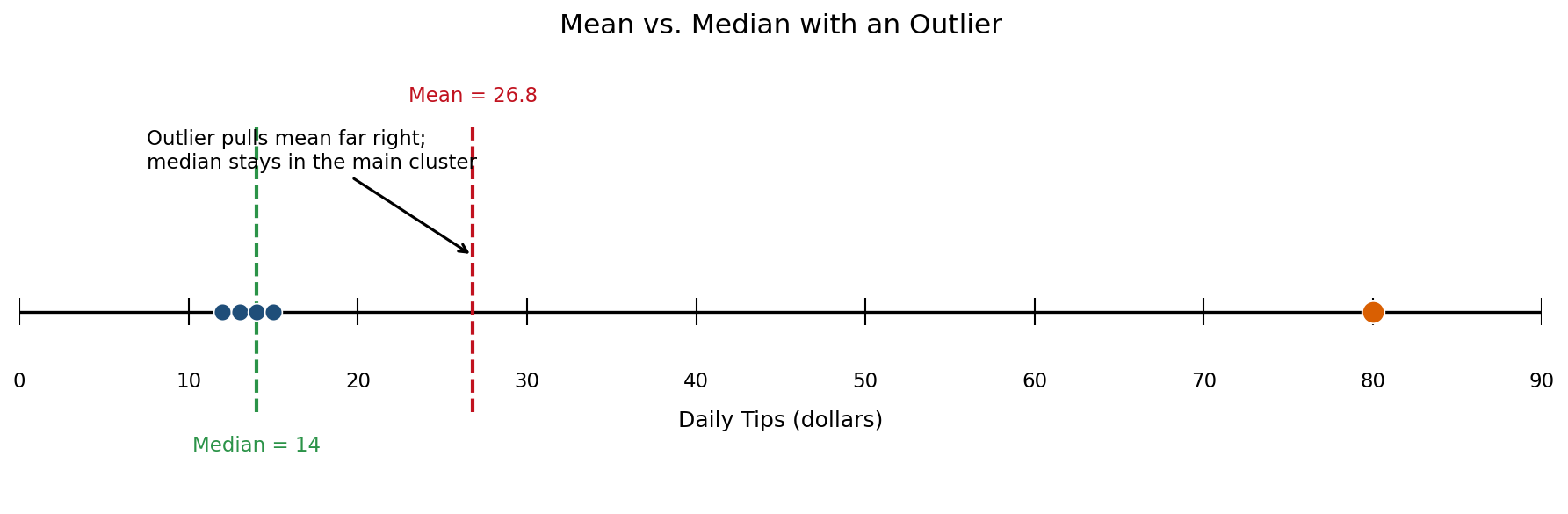
For example, imagine recording the daily tips a barista earns over five shifts:

Most values cluster between $12$ and $15$, but sits far above. That is an outlier, and we are about to see exactly what it does to the mean.

Let's work through the numbers step by step. First, consider only the four typical shifts:

The mean is:

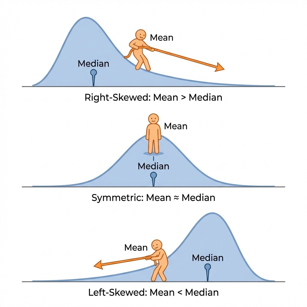
An outlier is a single extreme value, but sometimes an entire side of the distribution stretches out further than the other. When that happens, we say the distribution is skewed.

• A right-skewed (positively skewed) distribution has a long tail extending to the right. Most values cluster on the lower end, but a few high values pull the tail outward.
• A left-skewed (negatively skewed) distribution has a long tail extending to the left. Most values cluster on the higher end, but a few low values pull the tail outward.

A classic real-world example of right skew is household income. Most households earn moderate amounts, but a small number of very high earners stretch the distribution to the right. Test scores on a very easy exam, where most students score high but a few score low, would be an example of left skew.

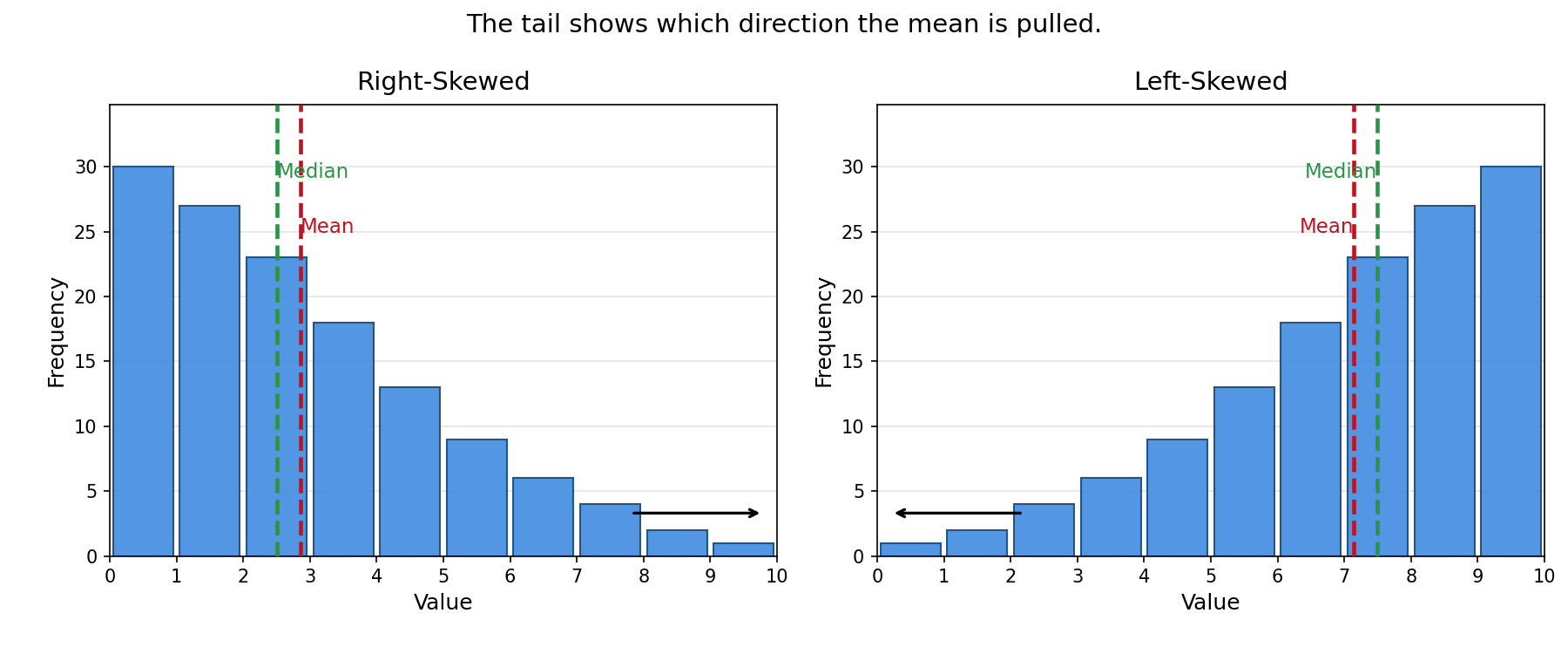
Skew acts on the mean in the same way an outlier does, just spread across many values in the tail rather than concentrated in a single point. The tail contains values that are far from the center, and the mean absorbs all of them into its calculation. The median, as always, holds its ground near the middle position.

Let's tie both ideas together with one more example. Suppose we have home sale prices (in thousands of dollars) for a small neighborhood:

Five of the six prices cluster between $220$K and $250$K, but K is a luxury property far above the rest. The mean is:

In this lesson, we explored how outliers and skewed distributions pull the mean away from the median. Because the mean includes every value in its calculation, even one extreme number can shift it dramatically, while the median depends only on the middle position and remains stable. We also learned a handy rule: the mean chases the tail, shifting toward whichever side the distribution stretches.

Now it is time to put these ideas to the test! In the upcoming practice exercises, you will predict how outliers move the mean, crunch the numbers to see the shift firsthand, and explain in your own words why one measure of center can paint a more honest picture than another. Jump in and see how sharp your intuition has become!