In the previous lesson, you prepared your ingredients: Query A (the high-velocity time-series data from server_load) and Query B (the static lookup data from server_owners). You ensured they shared the identical "Join Key": hostname.

Now, it's time to move from the Queries tab to the Transformations tab.

This is where the magic happens. We are going to stitch these two separate data sources together, enrich our metrics with context, and clean up the result so it looks like a single, professional dataset. By doing this in the UI rather than SQL, you keep your dashboard fast and your logic easy to debug.

The first step in merging Query A and Query B is the Join by field transformation. Think of this as the UI equivalent of a SQL JOIN.

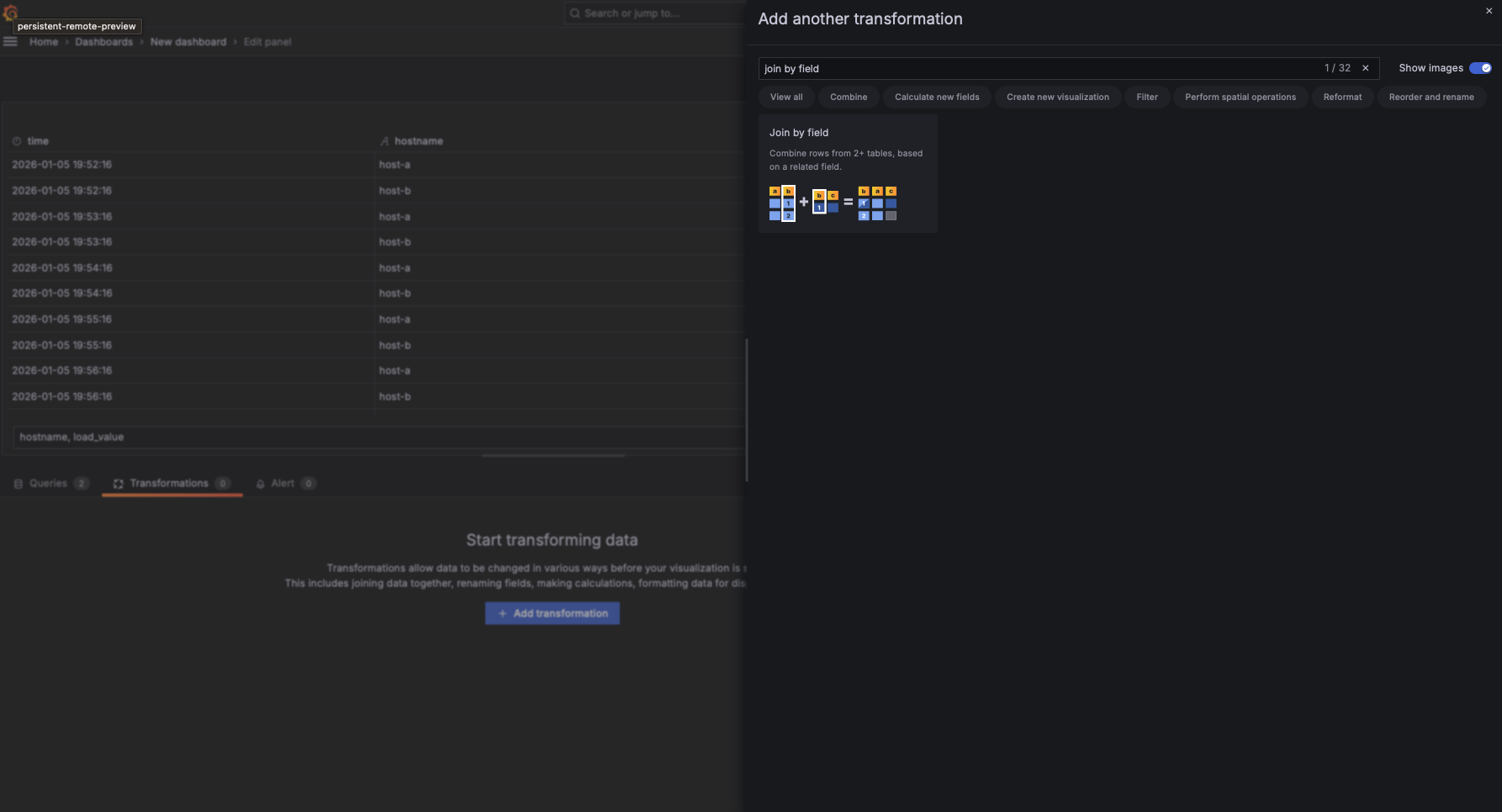
To get started, move to the Transformations tab (located next to Queries), click the Add transformation button, and search for "Join by field". When you select this transformation, Grafana looks at all the data currently loaded. Because you followed the "Join-Ready" rules (identical names and types), Grafana can automatically align the rows.

Once the transformation is added, you need to define how the data points should connect.

1. Select the Mode: Usually, you'll want "OUTER (TIME SERIES)". This ensures that even if a server is missing metadata in Query B, you still see its load metrics from Query A.
2. Select the Field: Choose the common identifier. In our server load example, you would select hostname.

Picking the right mode determines what happens when data is missing from one of your queries:

• INNER: Only shows rows where the join key exists in both Query A and Query B. If a server emits metrics but isn't in your lookup table, it will be hidden. Use this only if you want to strictly filter results to "documented" items.
• OUTER (TIME SERIES): The "Safe" default for metrics. It keeps all time-series data from Query A and simply appends metadata from Query B where it finds a match. If metadata is missing, the load metrics still show up with a null/empty team name.
• OUTER (TABULAR): Best for non-time-series data or when building a final "Report" table.
  • Pro-Tip: If you choose Tabular, you should go back to the Queries tab and ensure both Query A and Query B are set to Format: Table. Mixing a "Time series" formatted query with a "Table" formatted query in a Tabular join often results in duplicated rows or broken alignment.

Rule of Thumb: If Query A is metrics and Query B is lookup metadata $\rightarrow$ start with OUTER (TIME SERIES).

Why not do this in SQL?
By joining here, Grafana handles the "stitching" on the fly. If you decide to add Query C (like server "Location" or "Environment") later, you just add another small query and include it in the join. No complex SQL subqueries required.

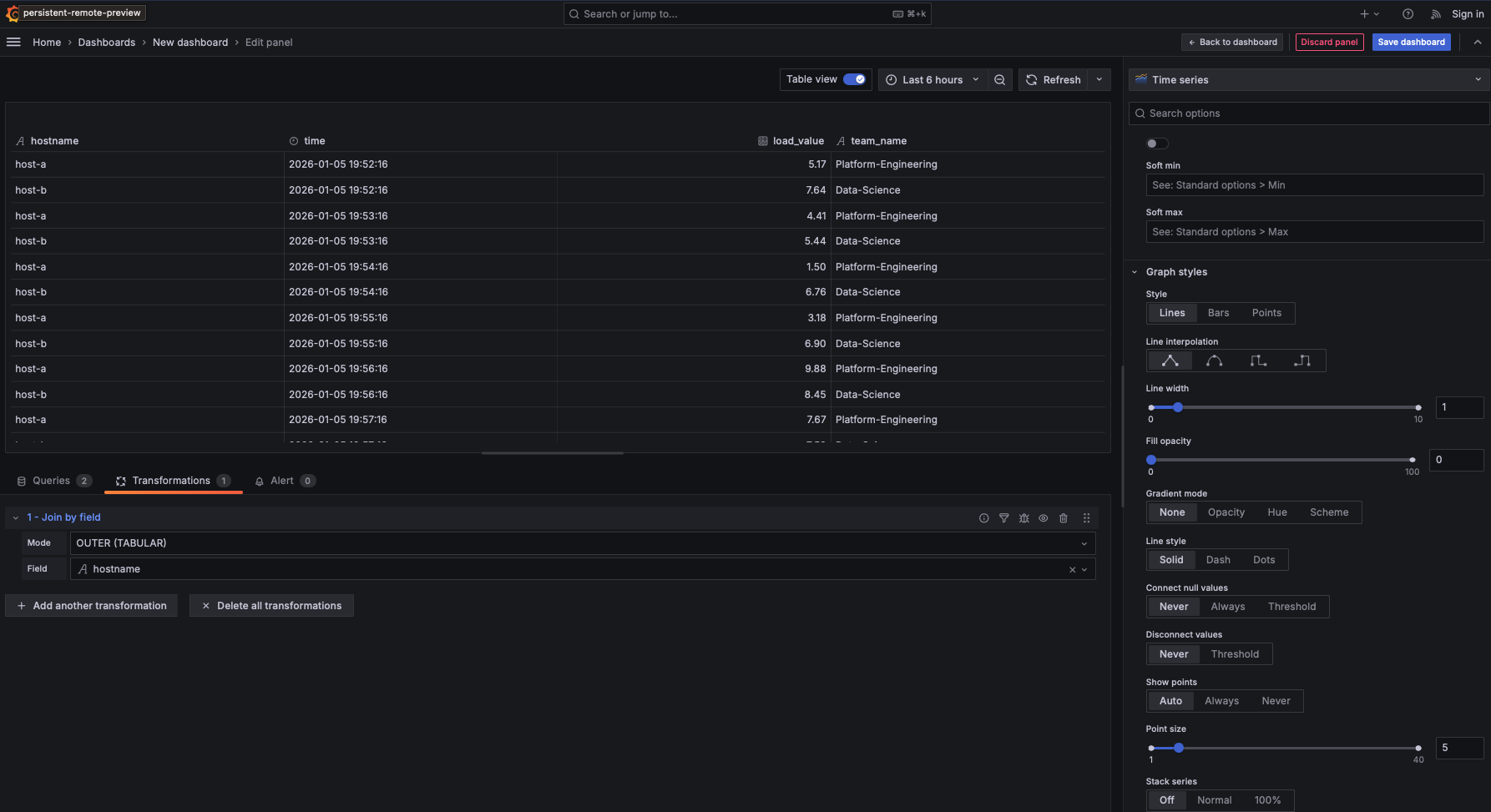
After the join completes, your table now contains columns from both queries in the same view:

• Time (from Query A's $__time() macro)
• hostname (the join key)
• load_value (from Query A)
• team_name (from Query B)

This is the core benefit of UI-based joins: you've enriched time-series metrics with contextual metadata without writing complex SQL. Now when you look at a spike in server load, you immediately see which team owns that server.

If your lookup table includes numeric fields (like capacity, thresholds, or budgets), you can use the Add field from calculation transformation to perform cross-source math. For example, if server_owners had a max_load_threshold column, you could calculate load_value / max_load_threshold to create a "% of Capacity" metric—all in the UI, without touching SQL.

Even with "Join-Ready" queries, things can go wrong. Here are the two most common issues you'll encounter in the Transformations tab:

1. The "Duplicate Column" Ghost: If you see hostname 1 and hostname 2, it means your join key names didn't match perfectly in the SQL (e.g., hostname vs host_name). Grafana treats them as different fields. Go back to your SQL and fix the AS alias.
2. Non-Unique Lookups: If Query B (server_owners) has two different rows for the same hostname, Grafana won't know which one to join to your metrics. The result will often look like "doubled" data. Ensure your Lookup Query is distinct.

By using Join by field, you have built a clean data pipeline entirely within the Grafana UI.

• Query A provided the heartbeat (Time and Load).
• Query B provided the context (Team Ownership).
• Transformations provided the assembly (Join and Polish).

This "Modular Design" is the secret to dashboards that are easy to maintain and incredibly fast.

In the upcoming practices, you'll perform this "Stitch and Enrich" workflow yourself. You'll take the server load data and join it with ownership metadata to create executive-ready views. Let's get to work!