Welcome to Grafana UI Joins and Transformations. In this lesson, we’re tackling a shift in mindset that separates basic dashboard builders from power users: Writing Join-Ready Queries.

In traditional database work, your instinct is to write a single, massive SQL query using JOIN statements to get all your data at once. While that works for reports, it’s often the "wrong" way to build high-performance monitoring dashboards. In Grafana, we prefer to keep our queries separate—one for the high-velocity metrics and one for the static reference data—and then stitch them together in the Transformation tab.

Why? Because joining a table with millions of rows of metrics to a table of metadata in SQL is resource-heavy and makes your queries brittle. By writing "Join-Ready" queries, you let the database do what it does best (fetch data fast) and let Grafana do what it does best (organize and visualize data).

To follow along, navigate to Dashboard -> New Dashboard -> Add visualization.

When writing join-ready queries, it is best practice to toggle the Table view switch at the top of the visualization area. While the final result might be a graph or a gauge, the Table view allows you to see the raw columns and data types as they arrive from the database. This is essential for verifying that your keys and aliases match perfectly before you move to transformations.

To make your queries work seamlessly within a dashboard, you need to use Grafana Macros. These are special functions that Grafana replaces with valid SQL right before sending the query to your database.

In the context of writing "Join-Ready" queries, two macros are absolutely essential:

1. The $__time() Macro:
When you fetch data from a database like PostgreSQL, the timestamp column might be in a format that Grafana doesn’t immediately recognize as the "X-axis" for a chart. By wrapping your timestamp column in $__time(your_column_name), you are telling Grafana: "This is the primary time sequence for this dataset."

Internally, Grafana converts this macro into a database-specific AS time statement. This is critical for joining data in the UI because it standardizes the time column across different queries. If Query A uses a raw timestamp and Query B uses a formatted one, the "Join by field" transformation might fail to align them on the timeline.

2. The $__timeFilter() Macro:
This is your primary tool for performance and precision. When a user changes the dashboard time range from "Last 24 hours" to "Last 15 minutes," the $__timeFilter(your_column_name) macro automatically updates your WHERE clause with the correct start and end times.

Why is this vital for UI-based joins?
Unlike SQL joins that happen on the powerful database server, Grafana Transformations happen in the user's browser. If your "Base Query" (Query A) accidentally pulls a million rows because it lacks a time filter, the browser will struggle to perform the join, leading to a laggy or crashed dashboard. Using $__timeFilter ensures that Query A only sends the exact slice of data needed for the current view, keeping the UI join fast and efficient.

To build a join-ready setup, you must categorize your data into two distinct types.

1. The Base (Query A): public.server_load
This is your time-series table. It tracks the actual performance metrics. Every minute, new rows are inserted for every host.

• Structure: It contains ts (timestamp), hostname (server name), and load_value (the metric).
• Scale: This table grows continuously and contains the bulk of your data.

2. The Lookup (Query B): public.server_owners
This is your static enrichment data. It stores reference information that rarely changes—like which department owns which server.

• Structure: It contains hostname and team_name.
• Scale: This table is tiny, usually containing only one row per unique server.

The Connection: Join Keys
The relationship is defined by the Join Key: hostname. By keeping these separate, we avoid repeating the "Team Name" for every single minute of data in a SQL join. We let each query do one job and let Grafana handle the assembly.

Our first query focuses on the raw load metrics. We need this query to provide the timeline and the key.

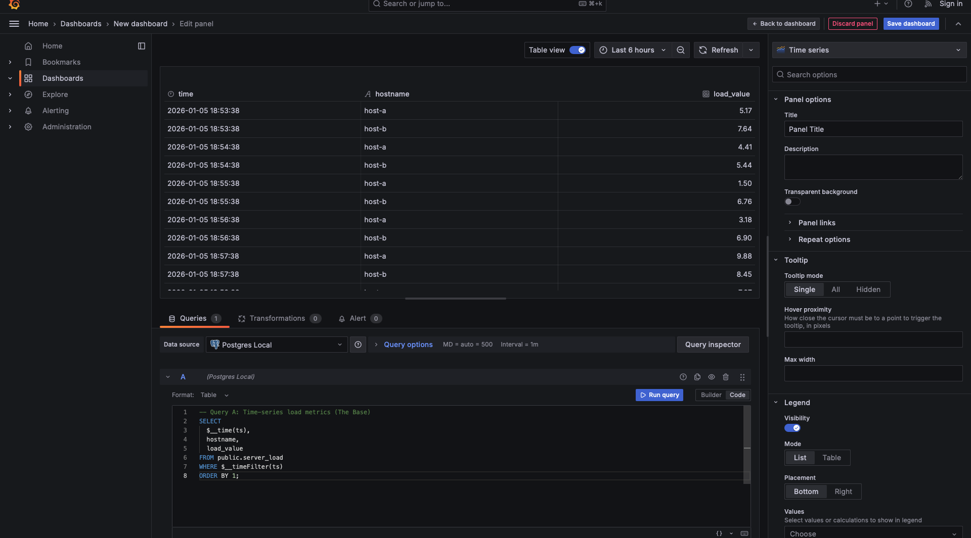
What makes this "Join-Ready"?
Notice that we explicitly included hostname. Even though we aren't "using" it for the Y-axis of a chart yet, it is the breadcrumb that allows Grafana to find the matching metadata in our next query.

Our second query is much leaner. It doesn't care about time; it only cares about the ownership of the servers.

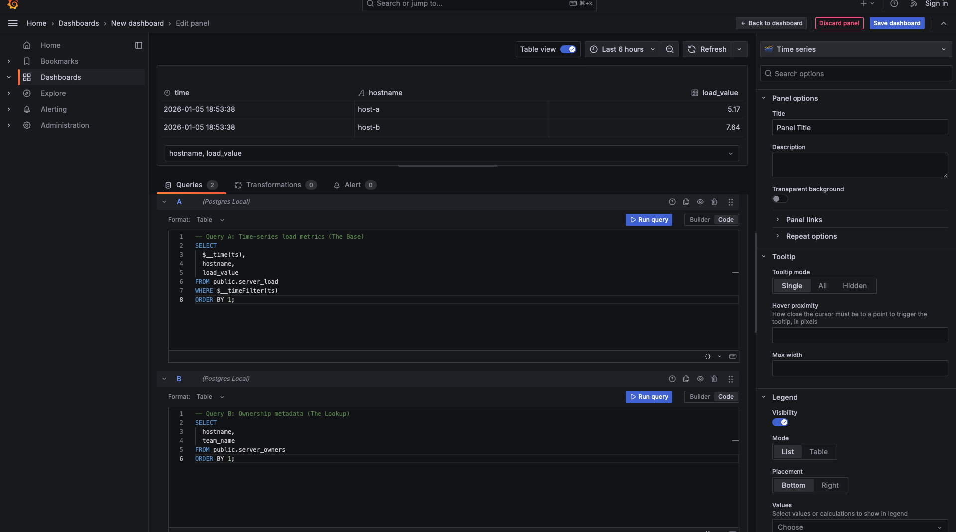
The "Magic" of Matching Names:
The most critical part of this query is the column naming. By selecting hostname with the exact same name as in Query A, we are signaling to Grafana’s Transformation tab that these columns represent the same entities. If Query A called it hostname and Query B called it server_id, Grafana wouldn't know they are the same thing without extra configuration.

When using a Time series panel, Query B does not appear in the panel preview — even in Table view. This is expected behavior.

Query B has no time column, so Grafana cannot render it independently in a visualization that requires a time axis. As a result, Grafana does not display Query B’s raw output in the preview at all.

This does not mean Query B is missing or ignored.

Even though it is not visible:

• Query B is executed
• Its data is loaded into the browser
• It is fully available to the Transformations pipeline

Once a transformation (such as Join by field) combines Query B with a time-series query, its fields become part of the final dataset and can then be displayed and visualized normally.

Before you move to the practice exercises, keep this checklist in mind. If your queries follow these rules, the Transformations in the next lesson will work every time:

1. Common Keys: Do both queries share a column that identifies the data (e.g., hostname)?
2. Identical Aliasing: Are those keys named exactly the same? (Case sensitivity matters!)
3. Type Consistency: Is hostname a string in both? If types differ, the UI join will fail.
4. Granularity: Does Query B provide a unique row for every key? If Query B has two different "owners" for the same host, the join results will become ambiguous.

You’ve now moved past the "one big SQL query" limitation. By writing focused, join-ready queries, you've created a modular data structure. Query A brings the "when" and "how much," and Query B brings the "who."

Get ready for the practice exercises—you're going to write these dual-query setups for a few different scenarios to ensure the "Join-Ready" logic becomes second nature!