In our previous lessons on Stitching Data, we joined datasets using a single unique identifier, like a device_id or a hostname. This works perfectly when one name equals one unique row of data. However, as you build more advanced dashboards, you will encounter scenarios where you need multiple pieces of information to identify a single metric. This is the "Multi-Field" Challenge.

Consider a Disk Usage dashboard:

• A single host (e.g., server-01) has multiple mount points (e.g., the root drive /, a database drive /var/lib/data, and a backup drive /mnt/backups).
• If you attempt to join your metrics to your inventory using only the host column, Grafana's transformation engine will see three different rows for server-01 and won't know which drive capacity belongs to which usage metric.

Since the Join by field transformation—which we introduced in the Stitching Data lesson—focuses on selecting one field to align data, we need a way to combine our identifiers.

The solution is the Composite Join Key.

A composite key is a single column created in your SQL query specifically to serve as a "hook" for Grafana's UI. We do this by concatenating (sticking together) multiple identifying fields into one unique string.

In PostgreSQL, we use the || operator to merge columns. By combining host and mount into a new column called join_key (e.g., server-01:/data), we provide Grafana with a single, unique string that aligns high-velocity metrics with static metadata perfectly.

The Workflow:

1. Query A (The Base): Pull the disk usage percentages and generate a join_key.
2. Query B (The Lookup): Pull the disk capacities and generate the exact same join_key.
3. The UI: Use this join_key to stitch the data together and then refine the view so the technical plumbing remains hidden from the user.

Our base query provides the heartbeat of the dashboard. We continue to use the $__time macros we established in the Writing Join-Ready Queries lesson to ensure the time-axis is formatted correctly for Grafana.

Pro-Tip: Why use the : separator?

Adding a character like : or - between your fields is a best practice. It makes the key easier to read during development and ensures that a host named web1 with a mount 01 doesn't accidentally collide with a host named web and a mount 101. Without the separator, both would appear as web101, causing the join to fail!

For our lookup query, we apply the same concatenation logic. As we learned in earlier lessons, this query does not require time macros because it handles reference data that remains static regardless of the dashboard's time range.

The Importance of Consistency

The transformation engine is literal. If Query A names the column join_key and Query B names it JoinKey, the UI will treat them as different fields. Precise naming is the secret to a successful data pipeline.

With both queries returning a join_key column, you can move to the Transform tab. This is where we use our "hook" to merge the high-frequency metrics with our static metadata.

Add the Join by field transformation

• Mode: Select Outer (TABULAR). This ensures that we keep all rows from our metrics and align them with the corresponding metadata, maintaining a tabular structure.
• Field: Select join_key.

Grafana will immediately align every row from Query A with its matching metadata from Query B. Because the join_key is unique to the host-mount pair, the data aligns perfectly without the ambiguity we faced earlier.

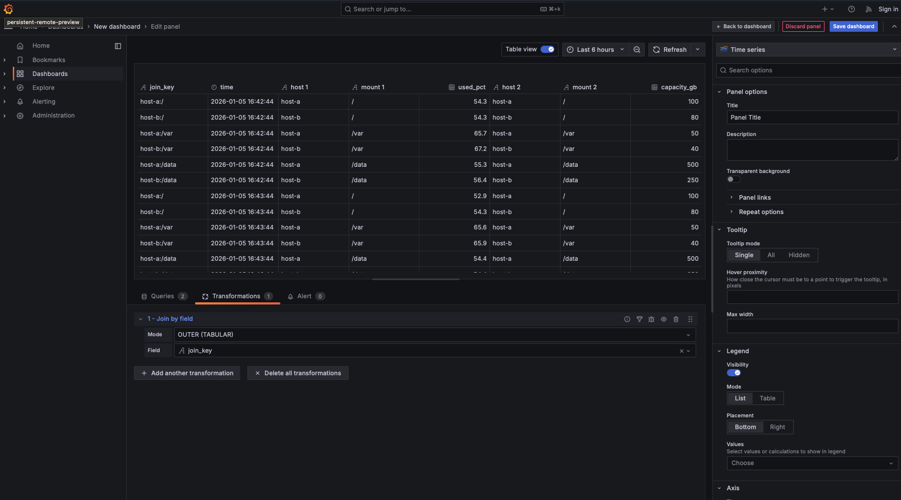
While the data is now joined, the table view is likely cluttered. You’ll see the join_key (which is for the machine, not the human) and duplicate host and mount columns from both queries. To fix this, we add a second transformation to curate the final user experience.

Add the Organize fields by name transformation

This specific transformation allows you to reorder, hide, and rename columns in a single interface.

• Hide the Join Key: Click the "eye" icon next to join_key. It has served its purpose as a technical "hook" and no longer needs to be visible to the end-user.
• Remove Duplicates: Use the "eye" icon to hide the extra host and mount columns that were pulled in from Query B to keep the table clean.
• Human-Friendly Labels: In the "Rename to" box, change the technical column names to something readable. For example, change used_pct to Disk Usage (%) and capacity_gb to Total Capacity (GB).

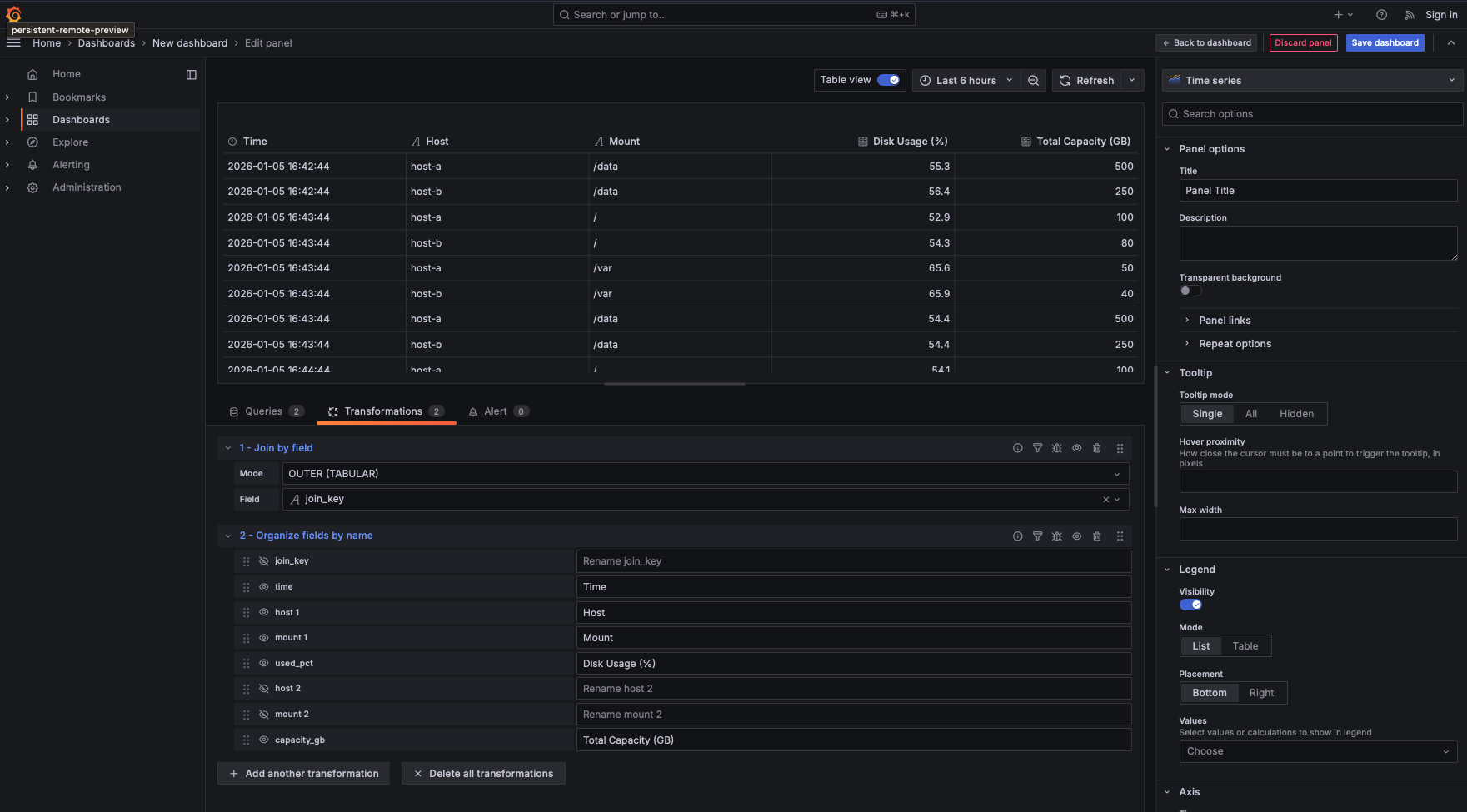
The final result is a professional dashboard displaying Time, Host, Mount, Usage %, and Capacity GB. By utilizing the transformation pipeline to hide the technical plumbing, the user sees only the context they need, while the "hook" logic remains functional but hidden behind the scenes.

Keep this checklist in mind for your upcoming exercises. If your queries follow these rules, your complex joins will work seamlessly:

1. Standardized Separator: Use the same separator (like :) in both queries.
2. Identical Order: Concatenate fields in the same order (e.g., always host then mount).
3. Unique Granularity: Ensure Query B has only one row per join_key. Duplicate keys in a lookup table will cause data to "double up" in the visualization.
4. Hide the Plumbing: Always use Organize fields to remove the join_key from the final panel. It is a developer tool, not a user-facing metric.

You have unlocked a significant power-up! You are no longer limited by the number of columns required to identify a specific data point. By creating Composite Join Keys in your queries and utilizing the Transformation pipeline to stitch and polish the data, you can build complex, high-performance dashboards that are both easy to navigate and easy to maintain. 🚀