Common Mathematical Symbols
Introduction
Welcome back to Writing Math in LaTeX — this is the seventh and final lesson of the course. Over the previous six lessons, we built up a powerful toolkit: math mode delimiters, subscripts and superscripts, fractions, square roots, standard function commands, and Greek letters. Together, those tools let us write a wide range of mathematical expressions. But if you have ever tried to type something like or , you may have noticed that the keyboard does not offer keys for symbols like or . In this lesson, we will learn the LaTeX commands for the most commonly used mathematical symbols — relational operators, set and logic notation, arrows, and special constants like infinity — and we will see how to track down less common symbols when the need arises.
Why Special Symbols Need Commands
Think about the symbols on a standard keyboard. We have +, -, =, <, and > readily available, and LaTeX happily uses them as-is inside math mode. However, mathematics relies on dozens of additional symbols — , , , , to name a few — that simply do not appear on any keyboard.
LaTeX handles these the same way it handles Greek letters: with backslash commands typed inside math mode. Just as \pi produces , a command like \infty produces . The names are typically abbreviated English words, so once you see the pattern, most commands feel intuitive. And because every symbol is just another command, it combines freely with the fractions, roots, subscripts, and function names we have already practiced.
Relational Operators
Relational operators compare two values. We already have <, >, and = on the keyboard, but mathematics uses several more. Here are the ones that appear most frequently:
| Command | Output | Meaning |
|---|---|---|
\leq | Less than or equal to | |
\geq | Greater than or equal to | |
\neq | Not equal to | |
\approx | Approximately equal to | |
\equiv | Identically equal to |
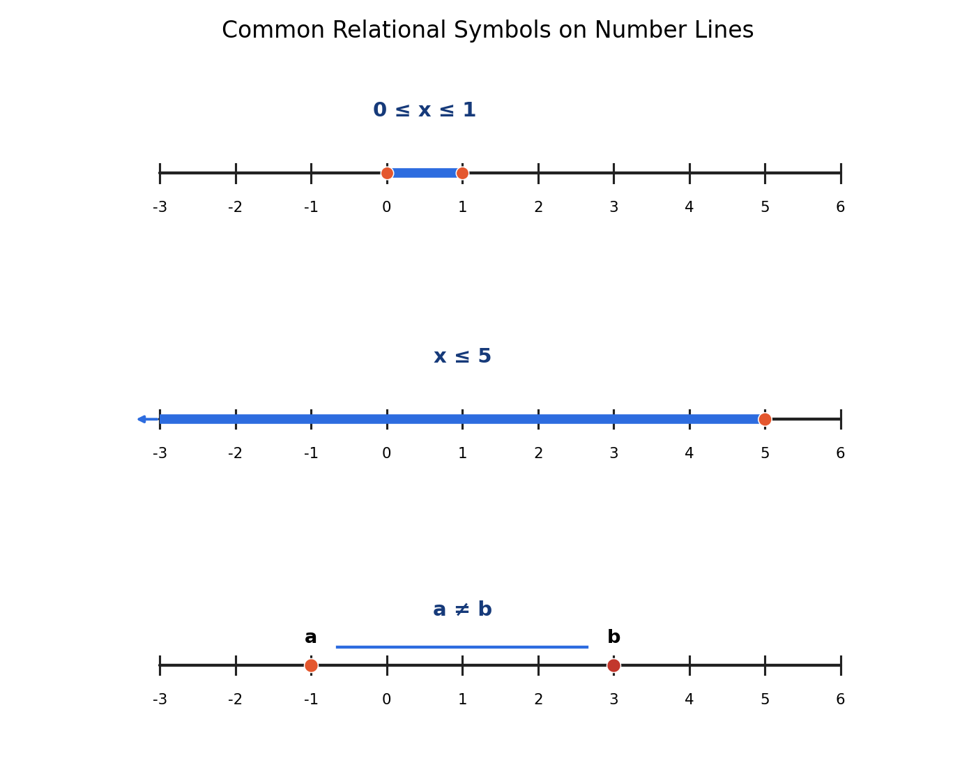
The command names are abbreviated forms of the English words: leq for "less or equal," geq for "greater or equal," neq for "not equal," and so on. This makes them relatively easy to remember. Here is a quick example using several relational operators together:
This produces , , and , with \qquad simply inserting a wide horizontal space between the examples. Notice how we chain \leq twice to express a range, and how \pi from last lesson fits naturally beside \approx. Every symbol is simply a command placed between the values it relates.
Set and Logic Notation
Set theory and logic have their own family of symbols. If you have taken a course in discrete mathematics or encountered Venn diagrams, many of these will look familiar. Let us start with the most common set symbols:
| Command | Output | Meaning |
|---|---|---|
\in | Element of | |
\subset | Proper subset of | |
\subseteq | Subset or equal | |
\cup | Union | |
\cap | Intersection | |
\emptyset | Empty set |
For logic, we have a parallel set of commands:
| Command | Output | Meaning |
|---|---|---|
\wedge | Logical AND | |
\vee | Logical OR | |
\neg | Logical NOT | |
\forall | For all | |
\exists | There exists |
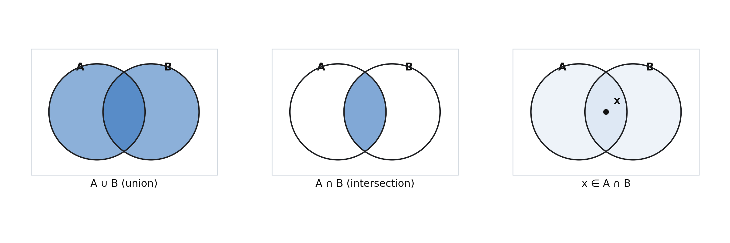
A helpful way to remember the set operations: \cup looks like a cup (, for union), and \cap looks like a cap (, for intersection). For the logic operators, \wedge () points up like a tent for AND, and \vee () points down for OR. Here is an example that puts a few of these together:
This gives us , , and . Notice how the relational operator \neq from the previous section combines naturally with the set symbols — you can mix and match symbol families freely.
Arrows and Special Constants
Arrows show up constantly in mathematics to indicate mappings, implications, and logical equivalences. Here are the most useful arrow commands:
| Command | Output | Typical Use |
|---|---|---|
\to | Function mapping, limits | |
\rightarrow | Same as \to | |
\leftarrow | Reverse direction | |
\Rightarrow | Implies | |
\Leftarrow | Is implied by | |
\Leftrightarrow | If and only if |
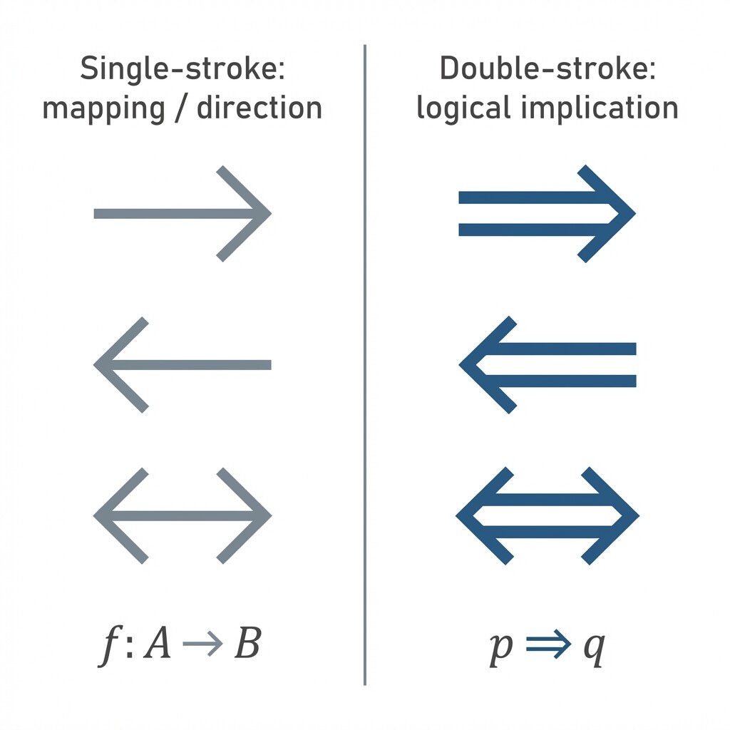
The pattern here is intuitive. Capitalizing the first letter gives a double-stroke (thick) arrow that signals logical implication, while the lowercase version gives a thin arrow used for mappings and limits. The command \to is simply a short alias for \rightarrow, so you can use whichever you prefer.
LaTeX also provides commands for a handful of special constants and operators that do not fit neatly into the categories above:
| Command | Output | Meaning |
|---|---|---|
\infty | Infinity | |
\pm | Plus or minus | |
\mp | Minus or plus | |
\times | Multiplication (cross) | |
\cdot | Multiplication (dot) |
You will see \infty most often in limits and intervals, while \pm appears in formulas like the quadratic formula. A quick example:
This produces (a function mapping from set to set ), (the statement " implies "), and (a measurement with its tolerance).
Symbols Working Together in Formulas
The real power of these symbols shows up when we combine them with each other and with the notation from earlier lessons. Let us walk through a few realistic examples.
A set definition using set-builder notation:
Here we use \in and \geq alongside a few new pieces of syntax: \{ and \} produce literal curly braces in the output, \mid produces a properly spaced vertical bar, and \mathbb{R} produces the blackboard-bold for the real numbers (this last command requires the amsfonts or amssymb package in your preamble). Do not worry about memorizing these extras right now — the key point is that our symbol commands mix seamlessly into larger expressions.
A logical implication with a relational chain:
This statement reads: "if and , then ." We combined \leq, \wedge, and \Rightarrow — relational, logic, and arrow symbols — in a single line.
Finally, a limit expression using \infty alongside the \lim command from Lesson 5:
The arrow \to indicates approach, and \infty serves as the target value. Together with \lim and \frac, we get a clean, publication-ready expression built entirely from tools covered in this course.
Looking Up Less Common Symbols
We have covered the symbols you will use most often, but mathematics has hundreds more — symbols for number theory, geometry, abstract algebra, and many specialized fields all have LaTeX commands. Nobody memorizes every one of them.
When you need a symbol that is not in our tables, two practical strategies will help:
- The Comprehensive LaTeX Symbol List is a well-known reference document that catalogs thousands of symbols with their commands and required packages. A quick internet search for "Comprehensive LaTeX Symbol List" will find it immediately.
- Detexify is an online tool where you draw a symbol with your mouse, and it suggests the matching LaTeX command. It is especially handy when you recognize a symbol visually but do not know its name.
With these resources in your back pocket, you will never be stuck searching for a symbol for long.
Conclusion and Next Steps
In this lesson, we learned how to produce common mathematical symbols in LaTeX: relational operators like \leq, \geq, \neq, and \approx; set notation with \in, \subset, \cup, and \cap; logic symbols including \wedge, \vee, and \neg; arrows such as \to, \Rightarrow, and \Leftrightarrow; and special constants like \infty and \pm. We also saw how these symbols combine with everything from earlier lessons to form complete, meaningful mathematical statements.
This brings us to the end of the lessons in Writing Math in LaTeX. Now it is time to put the full symbol toolkit to the test in the practice exercises, where you will write relational comparisons, set and logic expressions, and multi-symbol statements from scratch. Jump in and see how fluently you can speak the language of mathematical symbols!
