Sequential Updating
Introduction
Welcome back to Updating Beliefs and Surprising Results! You are now on lesson four of five, which means the finish line is well within reach. Over the first three lessons, we explored how the prior shapes the posterior, watched the false positive paradox unfold with rare conditions and accurate tests, and built the practical skill of spotting base-rate neglect in everyday arguments. Each of those lessons focused on a single update: one piece of evidence meets one prior, and out comes one posterior.
Real life, however, rarely stops at a single piece of evidence. A doctor orders a follow-up test. A second witness comes forward. Another data point arrives on our desk. In this lesson, we will learn sequential updating — the process of incorporating multiple pieces of evidence one at a time by letting each posterior become the prior for the next step.
Why One Update Is Rarely the End
Think about a routine medical checkup. A screening test comes back positive, so the doctor estimates a posterior probability that the patient has the condition. As we saw in earlier lessons, that posterior is often far lower than people expect, especially when the condition is rare. A single test result, no matter how accurate, may leave the question open.
So the doctor orders a second, confirmatory test. When that result arrives, we need a principled way to fold it into what we already believe. We could try to start over and somehow use both results at once, but that quickly becomes complicated. Sequential updating gives us a much cleaner path: handle one piece of evidence at a time, and let each answer build on everything that came before.
The Core Rule: Posterior Becomes Prior
The central idea is both simple and powerful. After we process the first piece of evidence with Bayes' theorem, we obtain a posterior probability. When a second piece of evidence arrives, that posterior steps into the role of the new prior. We then apply Bayes' theorem again, starting from the updated belief rather than the original base rate.
We can picture the chain like this:
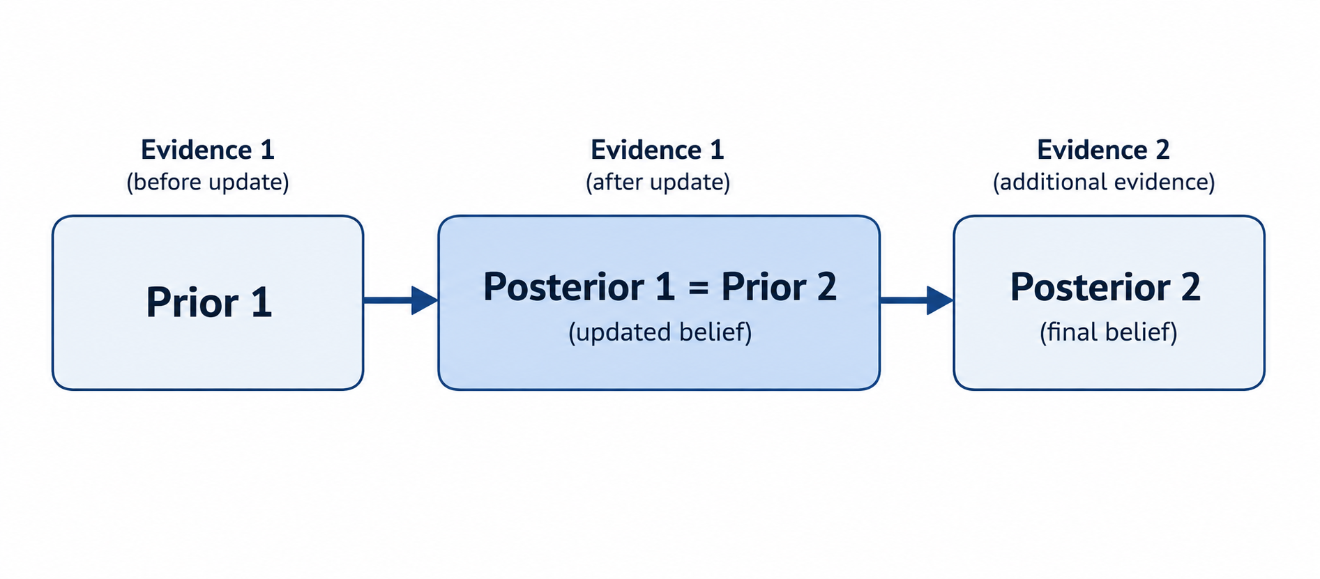
Each arrow represents one application of Bayes' theorem. The chain can extend as far as needed: a third piece of evidence would use as , and so on. The rule never changes: yesterday's posterior is today's prior.
Walking Through a Two-Step Update
Let us put numbers to this idea. Suppose a disease affects 1% of the population, so our initial prior is . A screening test has a sensitivity of 90% and a false positive rate of 5%:
Step 1 — First positive result.
We apply Bayes' theorem with the original prior. The denominator comes from the total probability of a positive result:
So the posterior after the first test is:
After one positive test, the belief in the disease rises from 1% to roughly 15.4%. That is a meaningful jump, but far from certain.
Step 2 — Second positive result.
The doctor orders a second, independent test with the same accuracy. Now our core rule kicks in: the posterior from Step 1 becomes the prior for Step 2.
New prior: , and .
We apply Bayes' theorem once more:
After two positive tests, our belief has climbed to about 76.6%. The full progression is summarized below:
| Stage | Prior | Evidence | Posterior |
|---|---|---|---|
| Start | 1.0% | First positive test | ≈ 15.4% |
| After test 1 | 15.4% | Second positive test | ≈ 76.6% |
Each row feeds into the next. The posterior on the right side of one row becomes the prior on the left side of the following row. That handoff is the entire mechanic of sequential updating.
Watching the Belief Climb
Notice what happened in the worked example. A single positive test moved our belief from 1% to about 15%. That was a large relative shift — the probability increased by a factor of 15 — but the posterior stayed fairly low because the base rate was so small. The second positive test, however, started from 15.4% instead of 1%, and that higher starting point made the same evidence far more powerful.
This illustrates a useful pattern: early evidence does the heavy lifting of overcoming a low base rate, while later evidence builds on a more favorable starting point. Each update compounds the effect, much like interest compounding on a growing balance. Two moderately strong pieces of evidence can, together, produce a high posterior even when neither one alone would have been convincing.
The General Pattern for Any Number of Updates
No matter how many pieces of evidence arrive, the procedure stays the same. Here is the recipe:
- Start with the initial prior, .
- Update using the first piece of evidence, , to get .
- Carry forward: set as the new prior.
- Update again using the next piece of evidence, , to get .
- Repeat for every additional piece of evidence that follows.
One important detail: the simplified step-by-step approach used here assumes that each new piece of evidence is conditionally independent of the earlier evidence, given the hypothesis. That lets us reuse the same likelihoods for each test after carrying the posterior forward. Sequential updating itself is more general: if evidence is dependent, we can still update in order, but later likelihoods must condition on what was already observed, such as and , rather than reusing fixed rates. We will examine this independence assumption more closely in the next lesson. For now, the key takeaway is the carry-forward rule: every posterior becomes the next prior.
Conclusion and Next Steps
In this lesson, we learned the core mechanic of sequential updating: when multiple pieces of evidence arrive one after another, we do not start from scratch each time. Instead, each posterior steps forward as the new prior, and Bayes' theorem handles the rest. We walked through a two-step medical screening example and watched the belief in a disease climb from 1% to about 15% after one positive test, and then to roughly 77% after a second.
Now it is time to practice. In the exercises ahead, you will complete a two-step updating chain, compute posteriors at each stage, and explain the carry-forward reasoning in your own words. Let us turn this rule into second nature!
