Welcome to the world of DBSCAN (Density-Based Spatial Clustering of Applications with Noise)! In this lesson, we will explore the DBSCAN algorithm, a powerful clustering method that stands out for its ability to detect clusters of arbitrary shape and handle outliers effectively. Unlike some clustering algorithms, DBSCAN does not require you to specify the number of clusters in advance. Instead, it groups data points based on density, identifying regions of high point concentration as clusters and labeling sparse regions as noise.

DBSCAN relies on two key parameters:

• Epsilon (Eps): The maximum distance between two points for them to be considered neighbors.
• Minimum Points (MinPts): The minimum number of points required to form a dense region (a cluster).

In this lesson, you will learn the theory behind DBSCAN and implement it from scratch using C++. We will walk through each step, from creating a dataset to assigning cluster labels, using C++ data structures and syntax.

To begin, let's create a simple dataset of 2D points. In C++, we can represent this dataset using the Eigen library's MatrixXd type, which allows us to store numerical data in a matrix format. Each row of the matrix will represent a data point with two coordinates.

Here is how you can define a toy dataset in C++:

#include <Eigen/Dense>
using namespace Eigen;

int main() {
    // Define a dataset with 12 points, each having 2 coordinates (x, y)
    MatrixXd data(12, 2);
    data << 1, 2,
            1, 3,
            2, 2,
            8, 7,
            8, 8,
            25, 80,
            24, 79,
            25, 81,
            80, 25,
            81, 26,
            79, 24,
            89, 90;
    // ... (rest of the code)
}

This matrix contains 12 points in 2D space, which we will use for clustering.

Before running DBSCAN, we need to assign initial labels to each point. In DBSCAN, points can be classified as:

• Noise (outlier): Points that do not belong to any cluster (label 0).
• Cluster members: Points that belong to a specific cluster (labels 1, 2, etc.).

We will use a std::vector<int> to store the label for each point, initializing all labels to 0 (noise). We also need to determine which points are core points (points with at least MinPts neighbors within Eps distance) and which are not.

Here is how you can implement this step in C++:

#include <vector>
#include <set>
using namespace std;

// data: MatrixXd containing the dataset
// Eps: maximum distance for neighbors
// MinPts: minimum number of neighbors to be a core point

vector<int> dbscan(const MatrixXd& data, double Eps, int MinPts) {
    int n = data.rows();
    vector<vector<int>> point_count(n); // Stores neighbors for each point
    vector<int> point_label(n, 0);      // Stores cluster label for each point
    set<int> core;                      // Indices of core points
    set<int> noncore;                   // Indices of non-core points

    // For each point, find neighbors within Eps distance (including itself)
    for (int i = 0; i < n; ++i) {
        for (int j = 0; j < n; ++j) {
            if (euclidean_distance(data.row(i), data.row(j)) <= Eps) {
                point_count[i].push_back(j);
            }
        }
        // Classify as core or non-core
        if (point_count[i].size() >= MinPts) {
            core.insert(i);
        } else {
            noncore.insert(i);
        }
    }
    // ... (clustering step follows)
}

This code checks each point and counts how many points are within the Eps radius. If a point has at least MinPts neighbors, it is considered a core point.

Now that we have identified core points, we can assign cluster labels. The process is as follows:

1. For each unvisited core point, assign a new cluster label.
2. For each neighbor of this core point, if it is not yet labeled, assign it to the current cluster.
3. If a neighbor is also a core point, repeat the process for its neighbors (using a queue for breadth-first search).
4. Continue until all reachable points are labeled, then move to the next unvisited core point.

Here is the C++ implementation of this step:

#include <queue>
using namespace std;

// ... (previous code)

    int ID = 1; // Cluster ID starts from 1
    for (int point : core) {
        if (point_label[point] == 0) {
            point_label[point] = ID;
            queue<int> q;
            for (int neighbor : point_count[point]) {
                if (point_label[neighbor] == 0) {
                    point_label[neighbor] = ID;
                    if (core.count(neighbor))
                        q.push(neighbor);
                }
            }

            // Expand the cluster
            while (!q.empty()) {
                int current = q.front(); q.pop();
                for (int neighbor : point_count[current]) {
                    if (point_label[neighbor] == 0) {
                        point_label[neighbor] = ID;
                        if (core.count(neighbor))
                            q.push(neighbor);
                    }
                }
            }
            ID++;
        }
    }

    return point_label;
}

This code ensures that all points in a dense region are assigned the same cluster label. Points that are not reachable from any core point remain labeled as 0 (noise).

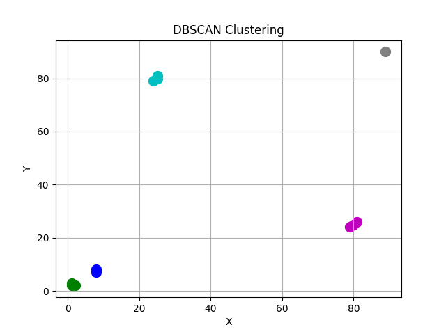
To better understand the clustering results, you can visualize the clusters using the matplotlibcpp library. Each cluster will be shown in a different color, and noise points will be shown in gray.

#include <matplotlibcpp.h>
namespace plt = matplotlibcpp;

// ... (after running dbscan and obtaining labels)

vector<string> colors = {"r", "g", "b", "c", "m", "y", "k"};
for (int i = 0; i < labels.size(); ++i) {
    int cluster = labels[i];
    string color = (cluster == 0) ? "gray" : colors[cluster % colors.size()];
    plt::scatter(std::vector<double>{data(i, 0)}, std::vector<double>{data(i, 1)}, 100.0, {{"color", color}});
}

plt::title("DBSCAN Clustering");
plt::xlabel("X");
plt::ylabel("Y");
plt::grid(true);
plt::save("static/images/plot.png");

This code will generate a plot of the clustered data and save it as an image:

Congratulations! You have learned the theory behind the DBSCAN clustering algorithm and implemented it from scratch in C++. You now know how to:

• Represent a dataset using C++ data structures.
• Compute Euclidean distances between points.
• Identify core points and noise based on density.
• Assign cluster labels using a density-based approach.
• Visualize clustering results.

You are now ready to apply DBSCAN to your own datasets and experiment with different parameter settings to discover meaningful clusters and outliers in real-world data.