Welcome back to Tree Diagrams and Decisions! You are now on lesson two of four in this course, so great progress so far. In the previous lesson, we built tree diagrams from scratch, carefully laying out nodes, branches, and paths for multi-stage experiments. Those structures showed us what could happen at each stage, but they said nothing about how likely each option was. In this lesson, we will complete the picture by assigning a probability to every single branch.
From Structure to Numbers
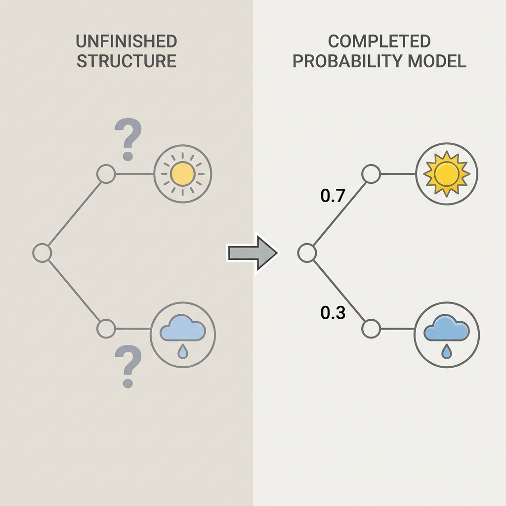
Consider a weather forecast. Knowing that tomorrow could be sunny or rainy is useful, but the real value comes from learning there is a 70% chance of sun and a 30% chance of rain. Tree diagrams work the same way. The skeleton we built last time tells us which outcomes are possible; the probability labels we add now tell us how likely each one is.
Once every branch carries a number, the tree becomes a full probability model. We can then calculate the likelihood of any specific outcome path, which will be the focus of our next lesson. For now, let us concentrate entirely on getting those branch labels right.
The Branch-Sum-to-One Rule
Labeling Branches for Independent Stages
Labeling Branches When Stages Are Dependent
Verifying Your Labels
Conclusion and Next Steps
In this lesson, we turned bare tree diagrams into complete probability models by labeling every branch with the correct value. The core principle is simple: branches leaving each node must sum to one. For independent stages, the same probabilities appear at every node within a given level, while for dependent stages we recalculate at each node using updated counts that reflect earlier outcomes.
Now it is time to put these skills to work! In the upcoming practice section, you will fill in missing probabilities, spot labeling errors, adjust for dependence in new scenarios, and build fully labeled trees from the ground up. Roll up your sleeves and let us see those branches add up!
Be a part of our community of 1M+ users who develop and demonstrate their skills on CodeSignal
At every node in a tree diagram, the experiment splits into all the possible outcomes for that stage. Because exactly one of those outcomes must happen, the probabilities on all branches leaving any single node must add up to 1:
P(branch1)+P(branch2)+⋯+P(branchn)=1
For instance, if a node has two branches labeled 0.3 and 0.7, the sum is 0.3+0.7=1.0 ✓. If three branches are labeled 0.5, 0.3, and 0.1, the sum is only 0.9 ✗, which signals a mistake. As you may recall from the first course in this path, the complement rule is handy here: when a node has just two branches, the second probability is simply 1 minus the first.
One important detail: this rule applies separately at every node. Different nodes in the same tree can have very different probability splits, and that is perfectly normal. The only requirement is that the branches from each individual node sum to one.
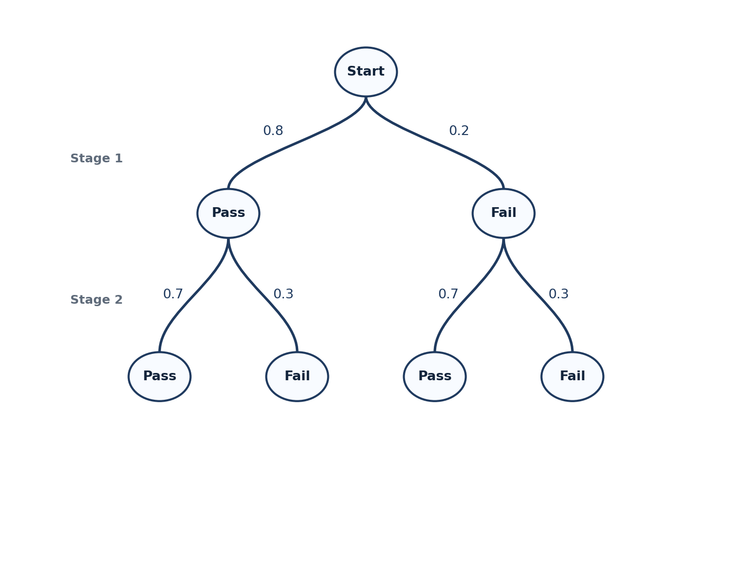
Let us start with the simpler situation: stages that do not influence each other. Suppose a student takes two short quizzes on unrelated topics. The probability of passing Quiz 1 is 0.8, and the probability of passing Quiz 2 is 0.7. Because the quizzes cover different material, the result of Quiz 1 has no effect on Quiz 2.
We label the tree stage by stage. At the root, Quiz 1 branches carry 0.8 for Pass and 1−0.8=0.2 for Fail. At every Stage 2 node, Quiz 2 branches carry 0.7 for Pass and 1−0.7=0.3 for Fail. The table below summarizes each node's labels and confirms the sum check.
Node
Pass
Fail
Sum Check
Stage 1 — Quiz 1
0.8
0.2
0.8+0.2=1 ✓
Stage 2 — Quiz 2
0.7
0.3
0.7+0.3=1 ✓
Because the stages are independent, every Stage 2 node receives the same pair of probabilities, no matter which Stage 1 branch we followed to get there. That visual symmetry across the second level of the tree is a clear indicator of independence.
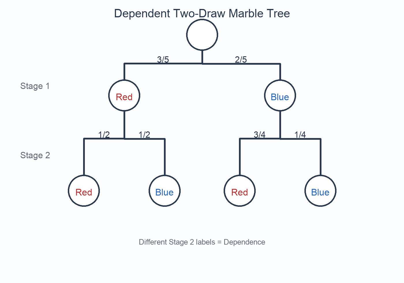
Now let us look at a situation where an earlier result changes the probabilities at the next stage. Imagine a bag holding 3 red marbles and 2 blue marbles. We draw one marble, set it aside without replacing it, and then draw a second.
Stage 1 begins with 5 marbles total, so the root branches carry 53 for Red and 52 for Blue. Stage 2 is where things get interesting. If the first marble was red, only 4 marbles remain — 2 red and 2 blue — so both branches from that node are 42=21. If the first marble was blue, 4 marbles remain but the mix shifts to 3 red and 1 blue, giving branches of 43 and 41. The table below lays out every node with its updated counts and labels.
Node
Items Remaining
Red Branch
Blue Branch
Sum Check
Start
3R, 2B (5 total)
53
52
1 ✓
After Red drawn
2R, 2B (4 total)
21
21
1 ✓
After Blue drawn
3R, 1B (4 total)
43
41
1 ✓
As you may recall from the previous course on how events influence each other, these Stage 2 values are conditional probabilities: each one is computed given the specific result of Stage 1. Notice that the second-stage nodes carry different labels — 21 and 21 after drawing red versus 43 and 41 after drawing blue. That asymmetry is the visual fingerprint of dependence. Whenever we draw without replacement, or face any scenario where an earlier outcome changes what is available, we must update both the numerator and the denominator before writing the branch labels.
Before calling a labeled tree complete, a quick three-step check can catch most errors:
Sum check at every node. Add the branch probabilities leaving each node. Every total must equal 1.
Denominator check. In dependent scenarios, confirm that the count of remaining items matches the denominator at each stage. For example, after removing one marble from five, the denominators at Stage 2 should all be 4.
Symmetry check. If stages are independent, same-level nodes should share identical branch labels. If stages are dependent, labels should vary and accurately reflect the updated conditions.
If any of these checks fails, trace back to the problem node and recalculate. Catching a labeling error now saves a lot of headaches when we begin multiplying along paths in the next lesson.