Welcome back to Tree Diagrams and Decisions! Lesson three of four means we are nearly at the finish line for this course. In the first two lessons, we built tree diagrams to map every possible outcome path and then labeled each branch with the correct probability. Those labeled trees hold all the information we need — now it is time to put those numbers to work. In this lesson, we will learn to calculate the probability of any specific outcome sequence by multiplying along its path through the tree.
From Labels to Likelihoods
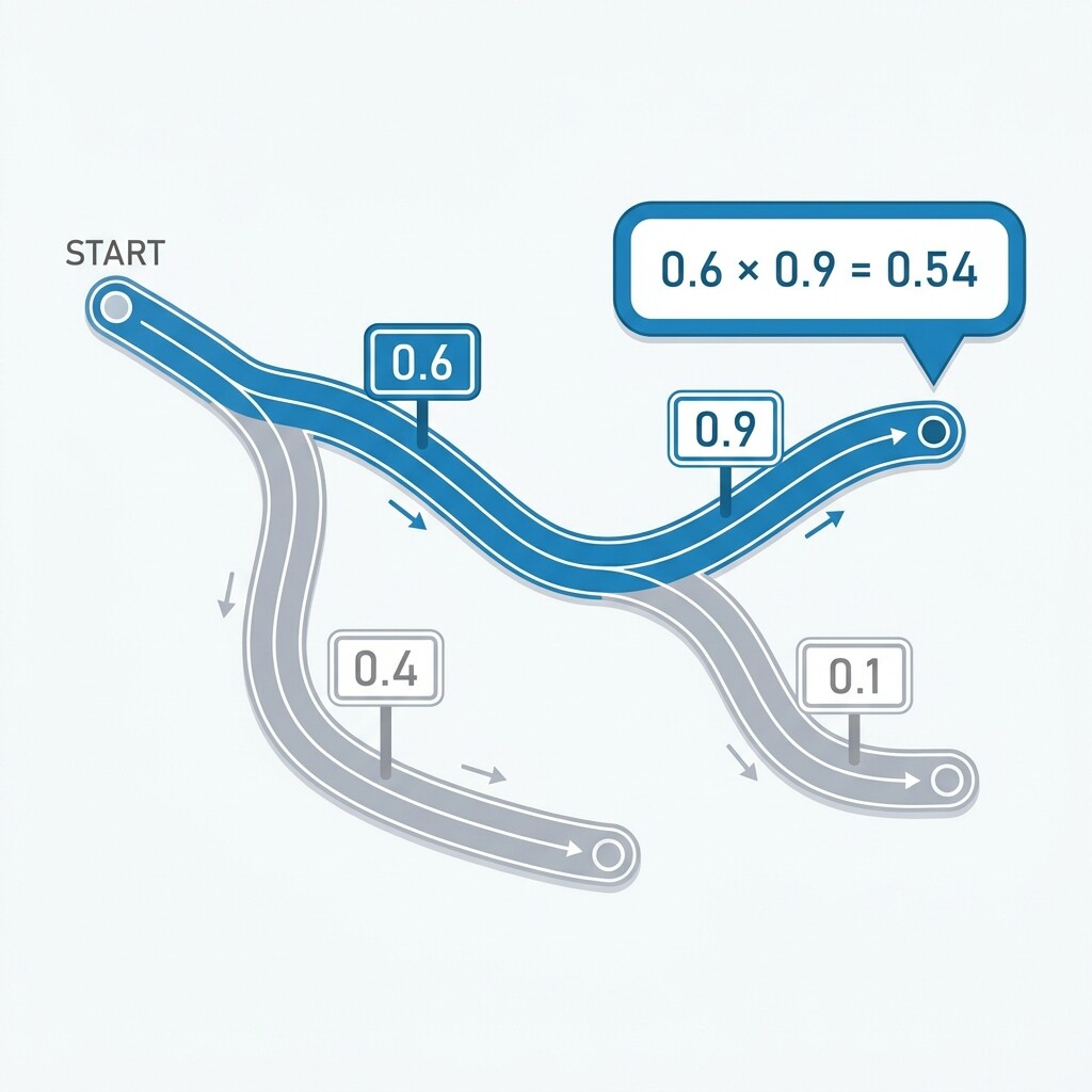
Picture a fully labeled tree diagram as a road map with distance markers on every road segment. The structure shows every possible route from start to finish, and the branch labels tell us how likely each individual segment is. To answer the question "How likely is this particular sequence of outcomes?", we need a way to combine the markers along that one route.
The tool for doing this is straightforward: multiplication. By multiplying the branch probabilities we encounter as we travel from the root node to a specific endpoint, we get the probability of that exact outcome sequence. Let us look at why this works and how to apply it step by step.
The Path-Probability Rule
Two-Stage Example: Movie Night
Path Probabilities with Dependent Stages
Comparing Paths Side by Side
Conclusion and Next Steps
In this lesson, we learned the path-probability rule: multiply all the branch probabilities along a path to find the probability of that specific outcome sequence. This rule works for both independent and dependent stages because the branch labels already encode the correct conditional probabilities. We also saw that comparing path probabilities is simply a matter of computing each product and checking which is larger — and that all path probabilities in a tree should sum to 1.
Now it is time to put your multiplication skills to the test! The practice exercises ahead will walk you through quality inspections, shipping logistics, sales funnels, and travel itineraries — each presenting a labeled tree with paths waiting to be traced and multiplied. Roll up your sleeves and let us start crunching those branches!
Be a part of our community of 1M+ users who develop and demonstrate their skills on CodeSignal
Here is the core rule of this lesson: to find the probability of a specific outcome sequence, multiply all the branch probabilities along that path.
P(path)=P(Stage 1 branch)×P(Stage 2 branch)×⋯
In practice, the calculation takes three quick steps:
Identify the specific outcome sequence you are interested in.
Trace the path from the root node through the matching branch at each stage.
Multiply the branch probabilities you encounter along the way.
Why does multiplication work here? Recall from the earlier course on how events influence each other that P(A and B)=P(A)×P(B∣A). When we labeled our branches in the previous lesson, each Stage 2 label was already set to the correct conditional probability given the Stage 1 result. So the branch labels are ready to be multiplied as-is — no extra adjustments needed, whether the stages are independent or dependent.
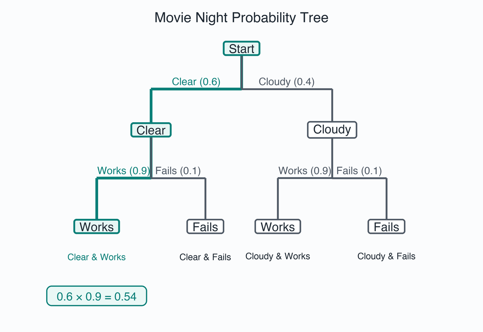
Let us see the rule in action with an independent scenario. A city park is hosting an outdoor movie night. The probability of clear skies is 0.6, and the probability that the projector works properly is 0.9. Weather and equipment are independent, so the projector probabilities remain the same regardless of sky conditions.
The tree diagram below shows the four possible paths. Suppose we want the probability that the evening goes perfectly: clear skies and a working projector. We trace that path from the root and multiply:
P(Clear and Works)=0.6×0.9=0.54
There is a 54% chance everything goes right. Now let us try the opposite path: cloudy skies and a projector failure.
P(Cloudy and Fails)=0.4×0.1=0.04
Only a 4% chance of the worst outcome. The process is identical for every path: start at the root, follow the branches that match your sequence, and multiply.
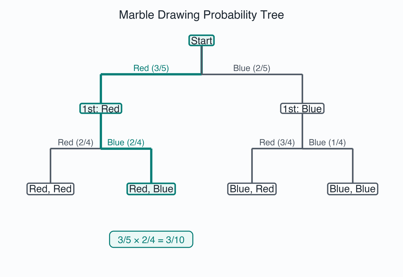
The multiplication rule works exactly the same way when stages depend on each other, because the branch labels already capture the updated conditional probabilities. Let us revisit the marble example from the previous lesson. A bag holds 3 red and 2 blue marbles, and we draw two without replacement.
We already labeled this tree: Stage 1 branches are 53 (Red) and 52 (Blue). After drawing red, Stage 2 shows 42 (Red) and 42 (Blue). After drawing blue, Stage 2 shows 43 (Red) and 41 (Blue). To find the probability of drawing red first and then blue, we trace that path and multiply:
P(Red then Blue)=53×42=206=103
We can also compute the path for blue first and then red:
P(Blue then Red)=52×43=206=103
The takeaway is that the process never changes: follow the path, multiply the branches. All the conditional adjustments are already built into the labels we assigned in the previous lesson.
Once we can calculate any single path's probability, comparing paths is straightforward: compute each product and see which is larger. Let us calculate all four movie night paths and lay them out in a table.
Path
Calculation
Probability
Clear → Works
0.6×0.9
0.54
Clear → Fails
0.6×0.1
0.06
Cloudy → Works
0.4×0.9
0.36
Cloudy → Fails
0.4×0.1
0.04
The perfect evening (Clear → Works) is the most likely single path at 0.54, while the total washout (Cloudy → Fails) is the least likely at 0.04 — more than thirteen times less probable. Notice that the four path probabilities add up to 0.54+0.06+0.36+0.04=1.00, which is a useful sanity check: every possible path has been accounted for, and exactly one of them must happen.
This kind of comparison is practical whenever we want to know which sequence of outcomes is most or least likely. It also sets the stage for the next lesson, where we will combine multiple paths to answer broader questions like "What is the total probability that the projector works, regardless of the weather?"