Welcome to the next step in your journey through the "Time Series Forecasting with LSTMs" course. In this lesson, we will focus on optimizing LSTM models to enhance their performance in time series forecasting tasks. As you may recall from previous lessons, LSTMs are powerful tools for capturing temporal dependencies in sequence data. However, they can be prone to challenges such as overfitting and long training times. In this lesson, we will explore various optimization techniques, including dropout, regularization, batch normalization, and early stopping, to address these challenges and improve model accuracy.

Overfitting occurs when a model learns not only the underlying patterns in the training data but also the noise and random fluctuations. As a result, the model performs exceptionally well on the training data but fails to generalize to new, unseen data. This leads to poor predictive performance in real-world scenarios.

Preventing overfitting is crucial because the goal of time series forecasting is to make accurate predictions on future or unseen data, not just to memorize the training set. Overfit models are less robust and can produce unreliable forecasts, which can be costly or misleading in practical applications. By applying techniques such as dropout, regularization, batch normalization, and early stopping, we help the model focus on the true patterns in the data and improve its ability to generalize.

Overfitting is a common issue in machine learning where a model performs well on training data but poorly on unseen data. One effective technique to combat overfitting is dropout. Dropout works by randomly setting a fraction of input units to zero during training, which helps prevent the model from becoming too reliant on any single feature. Let's see how to incorporate dropout into an LSTM model.

In this example, we define an LSTMModel class with a Dropout layer after the first LSTM layer. This means that 20% of the input units will be randomly set to zero during training, helping to reduce overfitting and improve the model's generalization ability.

Regularization is another technique used to prevent overfitting by adding a penalty to the loss function. In PyTorch, L1 and L2 regularization can be applied using weight decay in the optimizer. Let's see how to apply these regularization techniques to LSTM layers.

In this example, we apply L2 regularization by setting the weight_decay parameter in the optimizer. The regularization strength is set to 0.01, which is a common starting point. Regularization helps to constrain the model's complexity, reducing the risk of overfitting.

Batch normalization is a technique that normalizes the inputs of each layer to have a mean of zero and a variance of one. This helps stabilize and speed up training by reducing internal covariate shift. Let's see how to incorporate batch normalization into an LSTM model.

In this example, we add a BatchNorm1d layer after the first LSTM layer. This layer normalizes the output of the LSTM layer, helping to stabilize the training process and potentially improve convergence speed.

Early stopping is a technique used to prevent overtraining by monitoring the model's performance on a validation set and stopping training when performance stops improving. In PyTorch, this can be implemented manually by tracking the validation loss.

In this example, we implement early stopping by monitoring the validation loss. Training will stop if the validation loss does not improve for a specified number of epochs (patience), and the best model weights will be restored. This helps to ensure that the model does not overtrain and maintains good generalization performance.

With the optimization techniques in place, the next step is to compile, train, and visualize the performance of the optimized LSTM model. We will use the Adam optimizer and MSELoss function, which are well-suited for time series forecasting tasks. Additionally, we will visualize the training and validation loss over epochs and compare real versus predicted values to assess the model's performance.

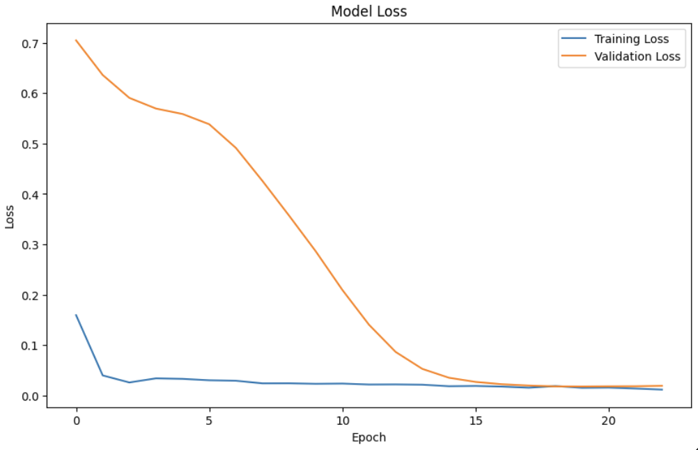
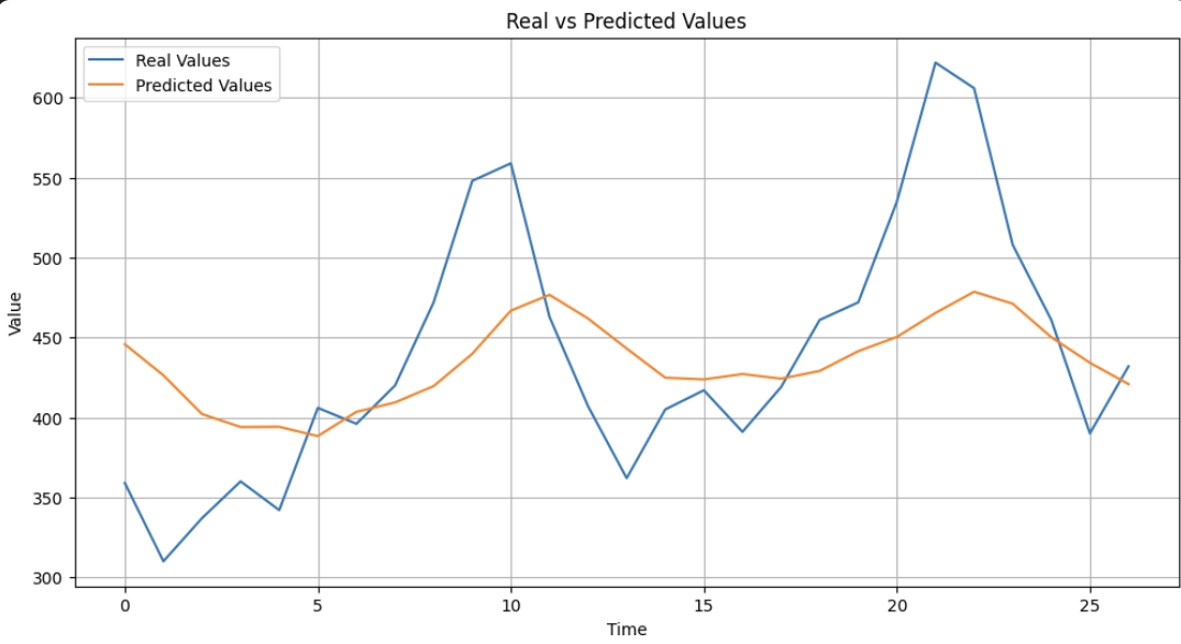
In this section, we first define the model, loss function, and optimizer. We then train the model using a custom training loop with early stopping. We visualize the validation loss over epochs using matplotlib, which helps in understanding the model's learning process and identifying any overfitting or underfitting issues. After training, we make predictions on the validation set and visualize the real versus predicted values to assess the model's performance. The plots are enhanced with grid lines and a larger figure size for better readability, providing a clear view of the model's accuracy in forecasting time series data.

The following plot shows how the validation loss changes over each training epoch. A decreasing loss indicates that the model is learning and improving its predictions.

This plot compares the actual values from the validation set with the values predicted by the optimized LSTM model.

In this lesson, we explored various techniques to optimize LSTM models for time series forecasting. We covered dropout, regularization, batch normalization, and early stopping, each of which plays a crucial role in enhancing model performance and preventing overfitting. As you move on to the practice exercises, I encourage you to apply these optimization techniques to your own LSTM models. Experiment with different parameters and datasets to deepen your understanding and improve your forecasting skills. This hands-on practice will solidify the concepts covered in this lesson and prepare you for more advanced topics in the course.