Welcome back to The Normal Distribution! This third lesson marks the midpoint of the course. In the first two lessons, we learned to recognize the bell shape and discovered that values cluster near the center while thinning out toward the tails. Those lessons treated every bell curve as one fixed picture — now it is time to ask: what controls how that picture looks?
The answer comes down to just two features — center and spread. Together, they completely determine the position and shape of any normal curve. By the end of this lesson, we will be able to explain what each feature controls and confidently compare two bell curves that differ in one or both of them.
Two Knobs on One Shape
Think of a bell curve as having exactly two "knobs" you can turn. One knob slides the entire curve left or right along the number line without changing its shape. The other knob stretches the curve wider or squeezes it narrower without moving its peak. Every normal distribution you will ever encounter is simply the result of setting these two knobs to particular values.
This is one of the reasons the normal distribution is so widely used: no matter how different two datasets look, if both follow a bell shape, they differ only in where the bell sits and how wide it is. Let's examine each knob on its own.
Center: Where the Bell Sits
The center of a normal distribution is the value directly below the peak. It marks the most common outcome and acts as the balance point of the curve. In statistics, we often call this value the mean and write it as μ (the Greek letter "mu").
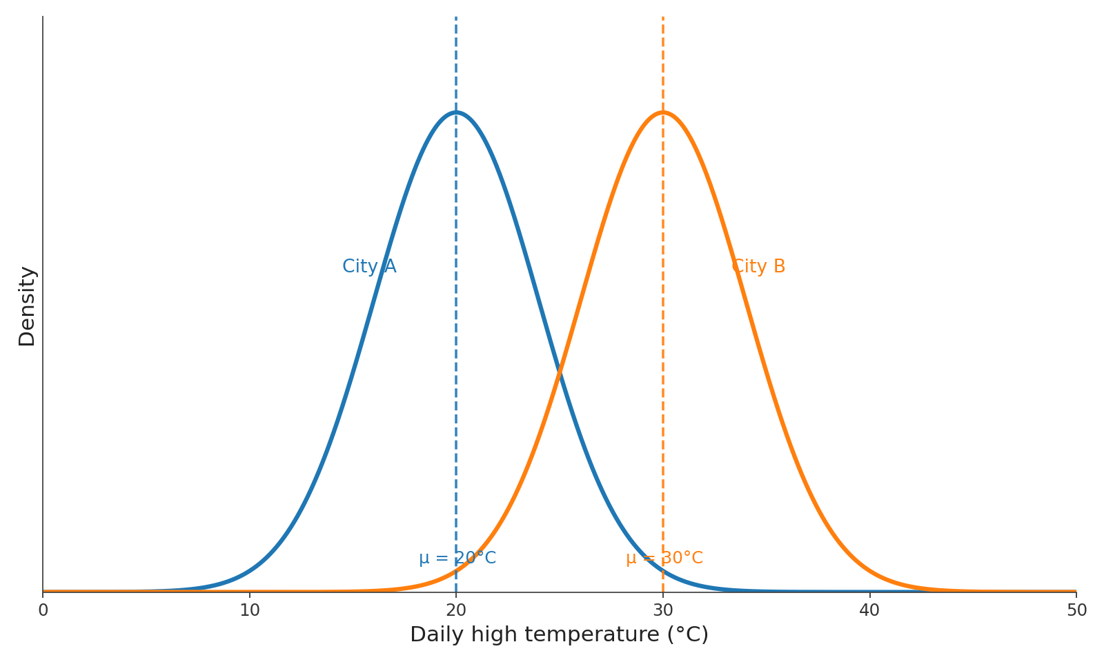
Changing the center slides the entire bell left or right. Imagine recording the daily high temperature in two cities during the same month. City A might have a bell centered at 20°C, while City B has a bell centered at 30°C. The two curves look identical in shape, but City B's curve sits 10 degrees to the right.
In the graph below, the two bells have the same spread but different centers.
A key point to remember: shifting the center does not change the curve's width or height. It only changes where the peak lands on the number line.
Join the 1M+ learners on CodeSignal
Be a part of our community of 1M+ users who develop and demonstrate their skills on CodeSignal
Spread: How Wide or Narrow the Bell Is
Center and Spread Are Independent
Comparing Two Bell Curves
When you place two normal curves side by side, you can describe how they relate by checking each feature separately:
Same center, different spread. The peaks line up at the same value, but one curve is wider than the other. Both groups share the same typical value, yet one group's data varies more.
Different center, same spread. The curves have the same width but are shifted left or right relative to each other. Both groups are equally consistent, but their typical values differ.
Different center, different spread. The curves differ in both position and width. The groups have different typical values and different levels of consistency.
When you see two bells, ask yourself two questions: Are the peaks in the same place? and Are the curves the same width? The answers immediately tell you whether center, spread, or both differ.
The spread of a normal distribution describes how far values tend to stray from the center. A narrow bell means most values are tightly packed around the center; a wide bell means values are more scattered. The standard measure of spread is the standard deviation, written as σ (the Greek letter "sigma").
A smallσ produces a tall, narrow bell because nearly all values hug the center closely. A largeσ produces a short, wide bell because values wander farther from the center. Notice the tradeoff: when the curve stretches wider, its peak must drop lower so that the total area under the curve stays the same.
Here is a quick comparison to keep in mind:
Small Spread (σ)
Large Spread (σ)
Tall, narrow bell
Short, wide bell
Values tightly clustered
Values more scattered
Greater consistency
Less consistency
As we saw earlier when exploring spread, wider spread means less consistency. That same idea applies directly here.
One of the most important things to appreciate is that center and spread operate independently. Knowing where the bell sits tells us nothing about how wide it is, and knowing how wide it is tells us nothing about where it sits.
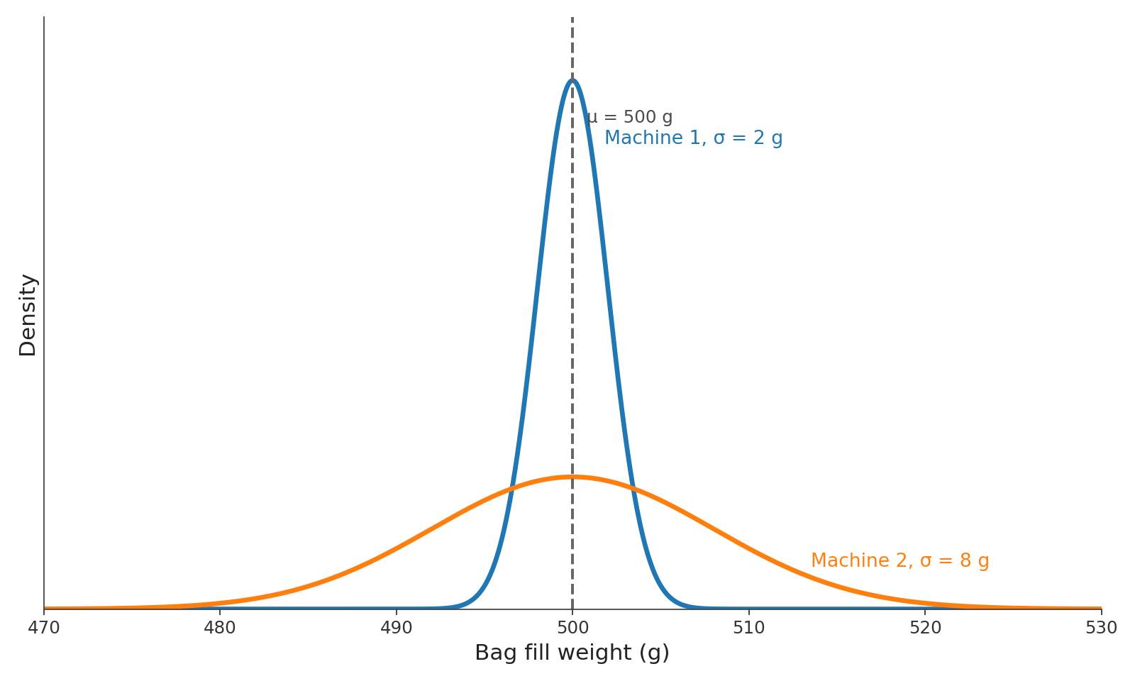
Consider two machines filling jars of honey. Both aim for 500 g, so both bells are centered at μ=500 g. However, Machine 1 has a spread of σ=2 g while Machine 2 has a spread of σ=8 g. The two curves share the same center, yet they look very different: Machine 1's curve is tall and narrow, and Machine 2's curve is low and wide.
The graph below shows the same center paired with two different spreads.
Same typical value, very different consistency — and that difference is entirely due to spread.
Suppose two coffee roasters each produce bags labeled as 250 g. We weigh a large number of bags from each roaster and plot the distributions.
Roaster A has a bell centered at μ=250 g with a spread of σ=3 g.
Roaster B has a bell centered at μ=255 g with a spread of σ=7 g.
What can we say? First, the centers differ: Roaster B's typical bag is 5 g heavier than Roaster A's. Second, the spreads differ: Roaster A's curve is narrower, meaning its bag weights are more consistent. If you value getting exactly the labeled weight with little variation, Roaster A is the more reliable choice.
Notice how much information we extracted just by comparing two numbers — μ and σ — for each curve. That is the power of understanding center and spread.
Every normal distribution is fully described by its center (μ), which sets where the peak sits, and its spread (σ), which sets how wide or narrow the bell is. These two features are independent: changing one leaves the other untouched. When comparing two bell curves, we simply check whether they differ in position, in width, or in both, and that tells us how the two groups' typical values and consistency relate.
Now it is your turn to put these ideas into practice. You will slide and stretch bell curves yourself, compare pairs of distributions, match curves to their descriptions, and write your own analysis of real measurement data. Let's jump in and make center and spread second nature!