Limits of Linear Correlation
Introduction
Welcome back to The Correlation Coefficient! We are now on lesson five of six, which means we are almost at the finish line for this course. Over the previous four lessons, we explored what represents, learned how to estimate it from scatter plots, standardized paired values, and computed from scratch.
In this lesson, we pause and examine a situation where relying purely on the number can lead us astray.
A Tool Built for One Job
As you may recall from the very first lesson, ranges from to and captures the direction and strength of linear association. It is specifically designed to detect patterns where points cluster around a straight line.
When the underlying relationship truly is linear, does a wonderful job condensing it into a single number. But not every real-world relationship follows a straight line. Some curve, bend, or even reverse direction partway through. In those situations, can paint a very incomplete picture.
When a Strong Pattern Hides from r
Imagine a study on the relationship between the amount of water provided to a plant each week and its observed growth. At low levels, more water is often associated with more growth. However, past a certain point, extremely high amounts of water are associated with a sharp drop in growth.
If we plotted watering amount on the horizontal axis and plant growth on the vertical axis, we would see an inverted U shape: growth levels are higher in the middle and lower at both ends. This is a clear, strong, and meaningful pattern.
Now think about what happens when we compute . On the left half of the curve, both variables increase together, so their z-score products are positive. On the right half, watering increases while growth decreases, so the products are negative. When we add all the products together, the positives and negatives largely cancel out. The result? A value of near zero, despite the obvious non-linear relationship in the data.
A Small Example
Let's see this play out with actual numbers. Consider five musicians tracked on daily practice hours () and a performance score ():
| Musician | (hours) | (score) |
|---|---|---|
| A | 1 | 3 |
| B | 2 | 7 |
| C | 3 | 8 |
| D | 4 | 7 |
| E | 5 | 3 |
The data shows a clear curve: performance scores are highest at moderate practice levels and lower at very high or very low levels. If we sketch these five points on a scatter plot, the curved shape is unmistakable.
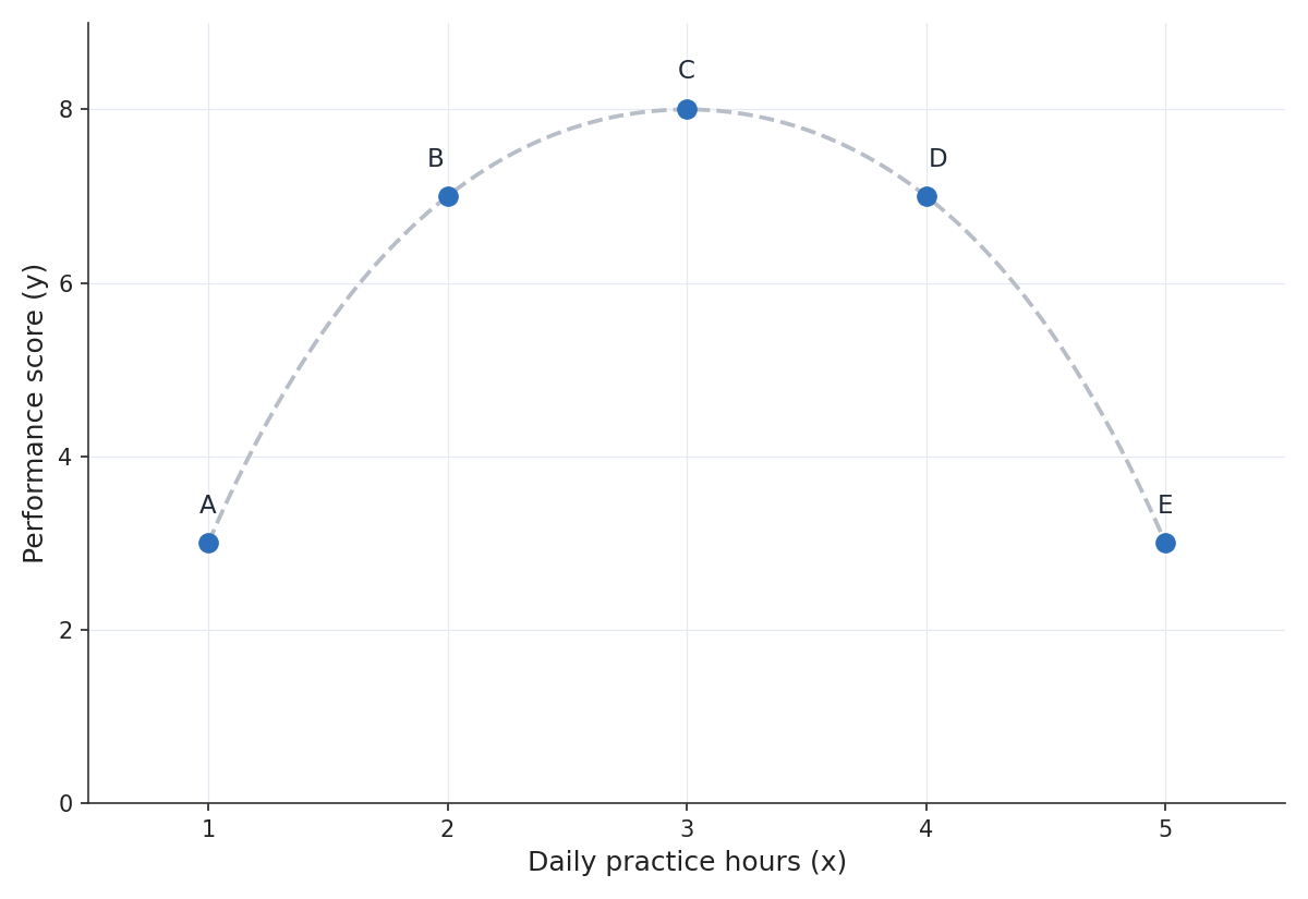
Yet if we compute , the sum of the z-score products is exactly zero, giving us . Someone who saw only that number might conclude that practice hours and performance have no relationship. But the scatter plot tells a different story: there is a strong connection; it just is not a straight line.
