You have reached the fourth lesson in The Binomial Distribution, putting you well past the halfway mark of this six-lesson course. Over the first three lessons, you built a solid foundation: the four requirements for a binomial setup, how to read the bar chart of success counts, and how the success probability p tilts the distribution left, right, or keeps it balanced. In each of those lessons, the number of trials stayed fixed while we focused on other features.
Now we shift attention to the other control in the binomial setup: the number of trialsn. What happens to the distribution when we keep p the same but run more trials? As you will see, changing n affects both where the bars concentrate and how widely they spread out.
A Quick Thought Experiment
More Trials Raise the Typical Count
Join the 1M+ learners on CodeSignal
Be a part of our community of 1M+ users who develop and demonstrate their skills on CodeSignal
Before we look at charts, let's build some intuition with a simple scenario. Imagine you flip a fair coin 5 times and count the heads. You would expect around 2 or 3 heads, and getting 0 or 5 would feel unusual but not shocking.
Now imagine flipping that same coin 100 times. You would expect roughly 50 heads, and getting 0 or 100 would be practically impossible. Notice two things happened when we moved from 5 flips to 100: the typical count jumped from about 2–3 up to about 50, and the range of realistic outcomes got wider. You would not be surprised by 45 or 55 heads out of 100, a span of about 10, whereas with 5 flips the realistic range covered only about 3 or 4 values. These two effects are the heart of today's lesson.
As you may recall from previous lessons, the peak of a binomial distribution sits near n×p. This product gives us the expected number of successes, and it grows in direct proportion to n. When we hold p fixed and increase n, the peak simply slides to the right.
Consider a process with p=0.30:
Number of trials n
Expected successes n×p
10
3
50
15
100
30
Every time we multiply n by some factor, the expected count multiplies by the same factor. Double the trials, double the typical count. This makes intuitive sense: if each trial has a 30% chance of success, running more trials simply gives that 30% more opportunities to produce a "yes."
More Trials Widen the Spread
Seeing Both Effects Side by Side
A Real-World Example: Small Survey vs. Large Survey
The center is only half the story. When we run more trials, the range of likely success counts also fans out. With n=10 and p=0.30, most outcomes land between roughly 1 and 5. With n=100 and p=0.30, typical outcomes might range from about 22 to 38. The cluster of likely counts covers a much wider stretch of values.
Why does this happen? Each trial adds a small bit of unpredictability — it might come up success or failure. The more trials we stack together, the more room there is for those small surprises to accumulate, which pushes some outcomes farther from the expected count. The spread of a binomial distribution is captured by the formula:
spread=n×p×(1−p)
You do not need to memorize this formula, but notice the key ingredient: n sits under the square root. That means the spread grows as n increases, but it grows at a slower pace than the center does. If we multiply n by 4, the center quadruples while the spread only doubles.
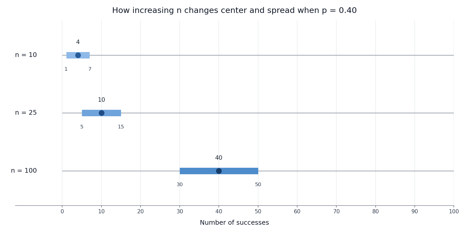
Let's put the two effects together in one comparison. Suppose p=0.40 and we look at three different trial counts:
In the table, the approximate likely range is built by taking the center plus or minus two times the spread, center±2×spread, and rounding to convenient whole-number endpoints.
Trials n
Center (n×p)
Spread (n×p×(1−p))
Likely range (approx.)
10
4
≈1.5
roughly 1 to 7
25
10
≈2.4
roughly 5 to 15
100
40
≈4.9
roughly 30 to 50
Reading down the table, both patterns are clear. The center climbs steadily, and the band of likely counts stretches wider. A bar chart for n=10 would be a tight little cluster of bars near 4, while a chart for n=100 would be a broader mound of bars centered around 40, spanning roughly 20 values instead of 6 or 7.
There is a subtle but important nuance here. The relative spread actually shrinks compared to the center: with n=10 the spread is about 38% of the center, while with n=100 it is about 12%. In everyday terms, the outcomes become less surprising as a percentage even though the raw range of counts gets larger. But when we look at the bar chart in absolute terms, we still have to scan more bars to cover the likely outcomes.
Imagine a company knows that p=0.20 of its customers reply "yes" to a satisfaction survey. A manager sends the survey to 10 customers on Monday and to 100 customers on Friday, then counts the "yes" replies each time.
For the Monday batch (n=10), the expected number of "yes" replies is 10×0.20=2. The likely range sits roughly between 0 and 4, a span of about 5 values.
For the Friday batch (n=100), the expected count jumps to 100×0.20=20. The likely range now stretches from about 12 to 28, covering around 17 values.
Both effects show up clearly: the larger group produces a higher typical count and a wider band of plausible counts. Consider what a result of 4 "yes" replies would mean in each case. On Monday, 4 out of 10 sits at the top of the likely range — high but not shocking. On Friday, 4 out of 100 would be far below the expected 20 and well outside the normal range. The same raw count tells a very different story depending on how many trials produced it.
In this lesson, we explored how the number of trials n shapes a binomial distribution when the success chance p stays fixed. Two effects work together: the center rises in direct proportion to n because n×p grows, and the spread widens in proportion to n, more slowly but still noticeably. More trials always mean both a higher typical count and a broader range of likely outcomes.
In the practice exercises ahead, you will compare distributions for small and large trial counts, judge how center and spread change, and apply your reasoning to a real survey scenario with two different group sizes. These tasks will help you build the habit of thinking about both effects whenever the number of trials changes.