Welcome back to The Binomial Distribution! So far in this course, you have learned what makes a process binomial and how to read the resulting bar chart — finding the peak, scanning the likely range, and spotting the rare counts in the tails. Now, in this third lesson, we ask a natural follow-up question: what happens to that bar chart when we change the probability of success?
Here we will explore how the success chancep reshapes the entire distribution. Adjusting p shifts where the bars pile up, tilting the distribution toward few successes, toward many, or balancing it right in the middle. By the end, you will be able to predict the shape of a binomial distribution just by knowing p.
The Success Chance as a Control Knob
Low Success Chance: Bars Lean Toward Few
Join the 1M+ learners on CodeSignal
Be a part of our community of 1M+ users who develop and demonstrate their skills on CodeSignal
Recall from the previous lesson that the peak of a binomial bar chart tends to sit near n×p. We saw this with 8 seeds at p=0.60, where the peak landed around 5, and with 10 light bulbs at p=0.90, where it landed at 9. In both cases, we held p fixed and read the chart. But what if we keep n fixed and varyp instead?
Think of p as a control knob that slides between 0 and 1. Turning the knob changes where the bars concentrate. A low setting crowds the bars toward the left (few successes), a middle setting centers them, and a high setting pushes them to the right (many successes). Let's walk through each scenario, all using n=10, so the only thing changing is p.
The comparison below shows this shift side by side.
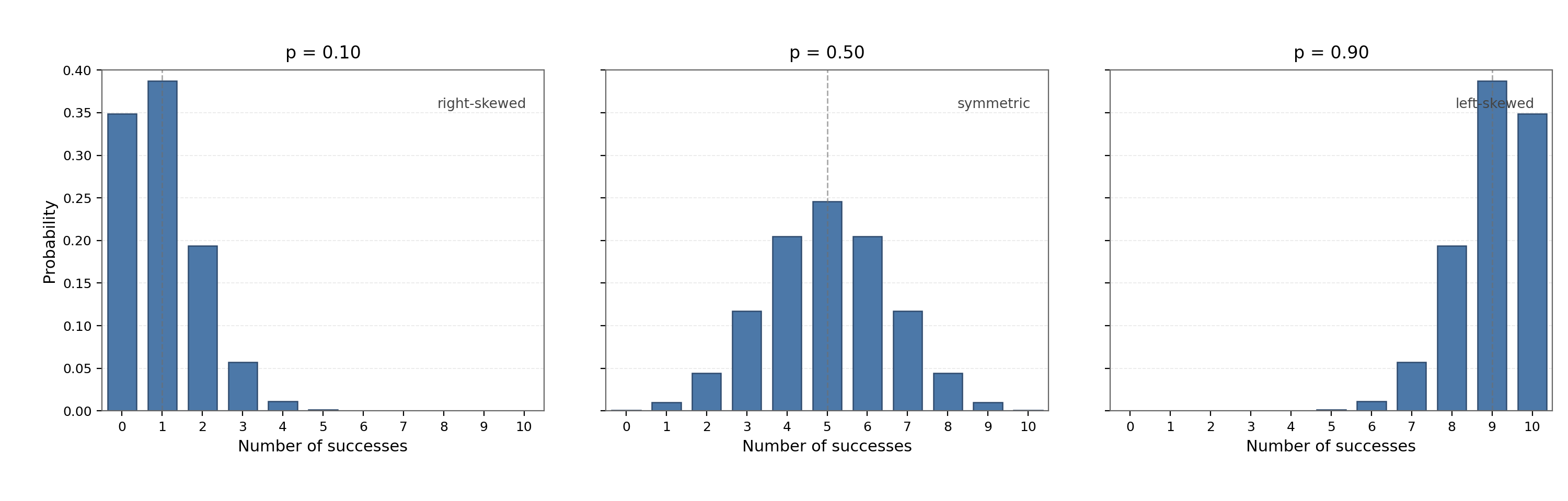
Suppose we flip n=10 coins, but each coin has only a p=0.10 chance of landing heads. Out of 10 flips, we expect about n×p=1 head on average. That single number already tells us a lot about the shape: the tallest bars will cluster near 0 and 1, and counts like 7, 8, or 10 will be almost impossible.
On the bar chart, the distribution leans heavily to the left. The bar at 0 is tall, the bar at 1 is the tallest or nearly so, and every bar after that drops off quickly. The right side of the chart is practically empty. You may notice that this creates a lopsided shape with a long, thin tail stretching to the right — a pattern called right-skewed (named after the tail direction, not where the bulk sits). When p is small, successes are hard to come by, so the bars bunch up near few successes.
Even Success Chance: Balanced in the Middle
High Success Chance: Bars Lean Toward Many
The Mirror Pattern
A Real-World Example: Free-Throw Shooting
Conclusion and Next Steps
In this lesson, we discovered that the success chance p acts as the main dial controlling the binomial distribution's shape. The product n×p points to where the peak will land, and the distance of p from 0.50 determines how lopsided the distribution is — the closer to even, the more balanced; the farther away, the more the bars lean to one side.
Up next, you will experiment with these ideas hands-on: adjusting the success chance, watching the distribution shift in real time, and predicting which way the bars will lean before they appear. Let's put your new intuition to the test!
Now turn the knob to p=0.50, keeping n=10. Each trial is equally likely to succeed or fail, like flipping a fair coin. The expected count of successes is n×p=5, sitting right in the center of the 0-to-10 range.
The bar chart reflects this balance perfectly. The tallest bar appears at 5, and the bars on either side taper down symmetrically — the bar at 4 and the bar at 6 are roughly the same height, and so are the bars at 2 and 8. When p=0.50, there is no reason for the distribution to favor the left or the right, so it sits centered and even.
Finally, slide the knob up to p=0.90. Now each trial almost always succeeds. With n=10, we expect about n×p=9 successes, so the tallest bars cluster near 9 and 10, while counts like 0, 1, or 3 are extremely rare.
This time the distribution leans heavily to the right. Most of the weight sits on the right side of the chart, and a thin tail trails off to the left. The shape is a mirror image of the low-p case: instead of right-skewed, it is left-skewed. When p is large, failures are uncommon, so the bars bunch up near many successes.
You may have noticed a neat symmetry in the examples above. A distribution with p=0.10 leans left, and a distribution with p=0.90 leans right, but their shapes are mirror images of each other. This is not a coincidence — calling something a "success" or a "failure" is just a label. If heads has probability 0.10, then tails has probability 0.90, so counting heads at p=0.10 produces the same shape as counting tails at p=0.90, just flipped.
Here is a quick summary of the overall pattern:
Success chance p
Peak near
Bars lean toward
Shape
Low (e.g., 0.10)
0 or 1
Few successes (left side)
Right-skewed
Even (0.50)
Middle (n/2)
Neither side
Symmetric
High (e.g., 0.90)
n−1 or n
Many successes (right side)
Left-skewed
“Toward few” does not mean that p must be close to 0; it means that p<0.50, so the center n×p lies below half of the trials. For example, with n=9 and p=0.35, the center is 9×0.35=3.15, so the distribution leans moderately toward fewer successes even though it is much less lopsided than the p=0.10 case.
The key takeaway: the closer p is to 0.50, the more symmetric the distribution; the farther p is from 0.50, the more the bars lean to one side.
Let's ground this in a concrete scenario. Imagine a basketball player who makes p=0.75 of her free throws. During warm-ups she takes n=12 shots. What shape should we expect for the number of successful shots?
The expected count of makes is n×p=12×0.75=9. Since p is above 0.50 but not extremely close to 1, the distribution will lean to the right, with the tallest bars around 8, 9, and 10. Low counts like 0, 1, or 2 will have tiny bars. The shape will be moderately left-skewed — p=0.75 is fairly high but leaves enough room for the occasional miss to pull some outcomes below the peak.
Notice how we reached this conclusion without any computation beyond 12×0.75. The value of p alone told us which direction the bars would lean and how lopsided the chart would look.