Welcome back to Stretching, Squeezing, and Reflecting Graphs! This is the second of three lessons, and it takes the idea of scaling and moves it to the other side of the function.
In the last lesson we ended with a warning: a vertically stretched parabola looks narrower, but nothing ever moved sideways. Today we meet the transformation that genuinely does move things sideways. The factor slips inside the parentheses, so it multiplies the inputs before the function ever sees them, and the new function is g(x)=f(kx).
There is a twist waiting for us. The effect of k on the picture runs opposite to what most people guess, and by the end of this lesson we will be able to predict and sketch f(kx) for large factors, small factors, and negative ones, with a solid reason for why the reversal happens.
Inside the Parentheses, Backwards Again
This is not the first time an inside change has caught us off guard. As you may recall from the horizontal shifts course, f(x−3) moves a graph three units to the right, even though the formula shows a subtraction. Anything that touches the input before the function processes it ends up acting in the opposite direction on the picture.
Multiplication follows the same pattern. A factor of 2 inside the parentheses does not make the graph twice as wide; it makes it half as wide.
A video played at double speed is the everyday version of this. Every scene still happens, at exactly the same volume and brightness — each one simply arrives at half its original timestamp, so the whole movie is compressed into a shorter stretch of time.
The Mapping (x, y) → (x/k, y)
Once again, the cleanest description of a transformation is a rule that says where each point goes. For g(x)=f(kx) with k=0, that rule is:
(x,y)→(kx,y)
The y-coordinate is copied over untouched, because k never reaches the output. It meets the input, gets multiplied in, and the function reports whatever value it would have reported for that product. Heights are preserved; only horizontal positions change, and they change by division, not multiplication.
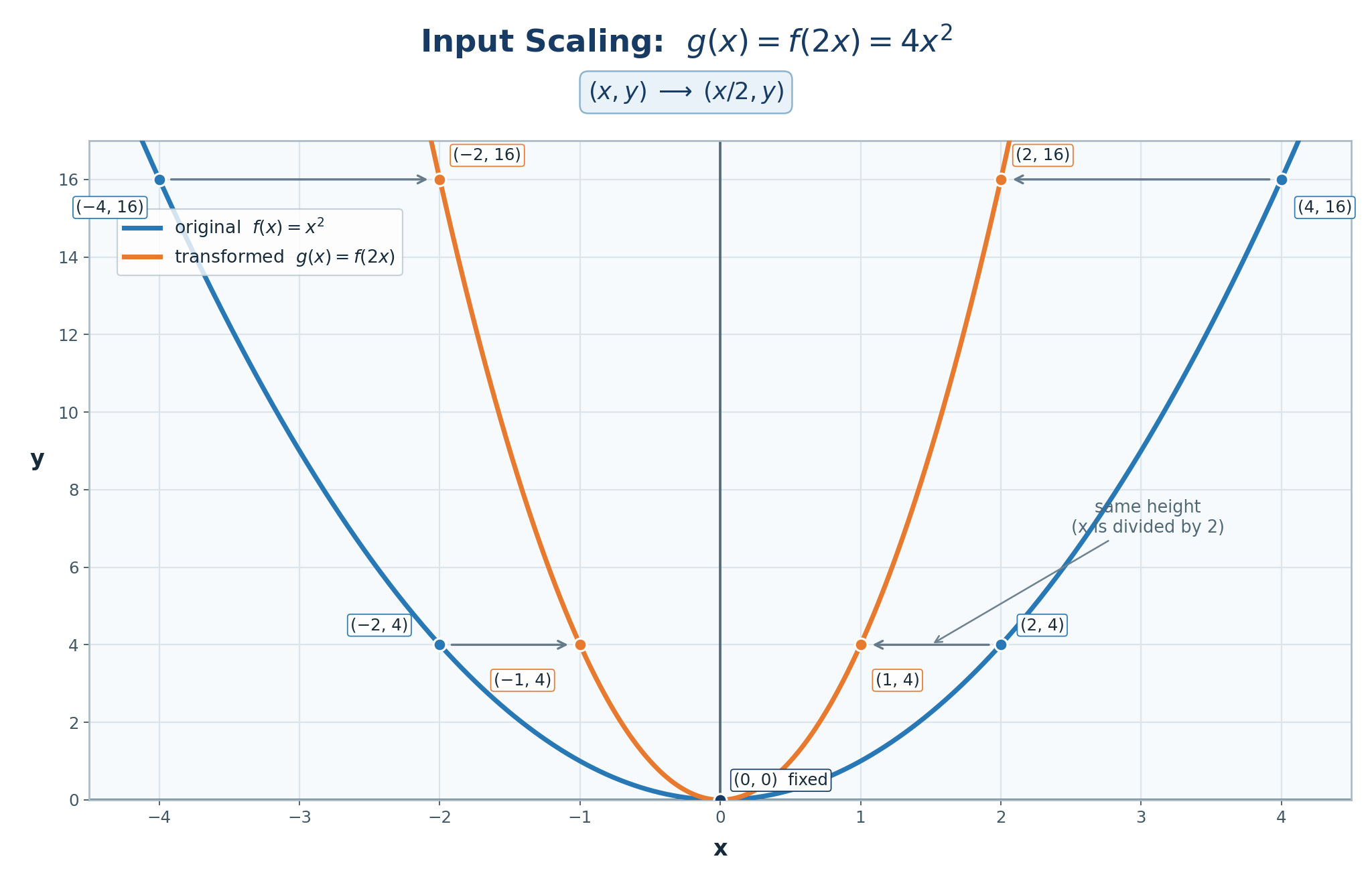
Let's apply this to f(x)=x2 with k=2, so g(x)=(2x)2.
Original point on f
Input f needed
New input x/2
New point on g
(−4,16)
−4
−2
(−2,16)
(−2,4)
−2
−1
(−1,4)
(0,0)
0
0
(0,0)
(2,4)
2
1
(1,4)
(4,16)
4
2
(2,16)
Every point stays at its own height and slides horizontally toward the y-axis, landing at half its original distance from it. The plot below makes those level, sideways movements easy to see.
Join the 1M+ learners on CodeSignal
Be a part of our community of 1M+ users who develop and demonstrate their skills on CodeSignal
Here is the argument that makes the reversal feel inevitable rather than strange. Pick any output of the original function, say f(4)=16 for f(x)=x2, and ask where the new function g(x)=f(2x) produces that same value.
We need the expression inside the parentheses to equal the familiar input:
2x=4⟹x=2
So g(2)=f(4)=16. The new graph reaches a height that the old one needed x=4 to reach, and it gets there already at x=2.
In general, solving kx=a gives x=a/k, which is exactly the mapping we wrote down. Doubling the input makes the function run through its values twice as fast, so the whole graph is pulled in toward the y-axis — a horizontal compression by a factor of 2.
The same reasoning with a small factor produces the opposite picture. Take f(x)=∣x∣ and k=31, so g(x)=31x. Dividing by 31 is the same as multiplying by 3, so the mapping sends (x,y) to (3x,y):
(−3,3)→(−9,3)
(−1,1)→(−3,1)
(0,0)→(0,0)
(3,3)→(9,3)
The V-shape keeps its vertex at the origin and still climbs to exactly the same heights, but it now needs three times as much horizontal room to get there. When 0<k<1, the graph is stretched horizontally, or widened.
Slow motion is the everyday version of this: the same events, at the same magnitudes, spread across three times as much time.
In both examples, the point (0,0) stayed exactly where it was, and that is no accident. One line of arithmetic explains it for every nonzero k:
g(0)=f(k⋅0)=f(0)
The new function and the old one always agree at x=0, so whatever the y-intercept was, it stays put. In mapping language, the same fact reads 0/k=0.
Points on the y-axis are the fixed points of any input scaling, and the y-axis behaves like the line the graph is squeezed toward or pulled away from — the same role the x-axis played for output scaling last lesson. That hands us a quick diagnostic to carry into the next lesson: if a graph has been scaled through its inputs, its y-intercept must be unchanged.
A negative factor splits into two familiar steps, just as it did for output scaling. Write the factor as its sign times its magnitude:
f(kx)=f(∣k∣⋅(−x))
The sign part is f(−x), which sends (x,y) to (−x,y). Each point keeps its height and moves to the mirror position on the other side of the y-axis, so this is a reflection across the y-axis. The magnitude part then squeezes or widens as usual, and since multiplication can be done in either order, so can the two steps.
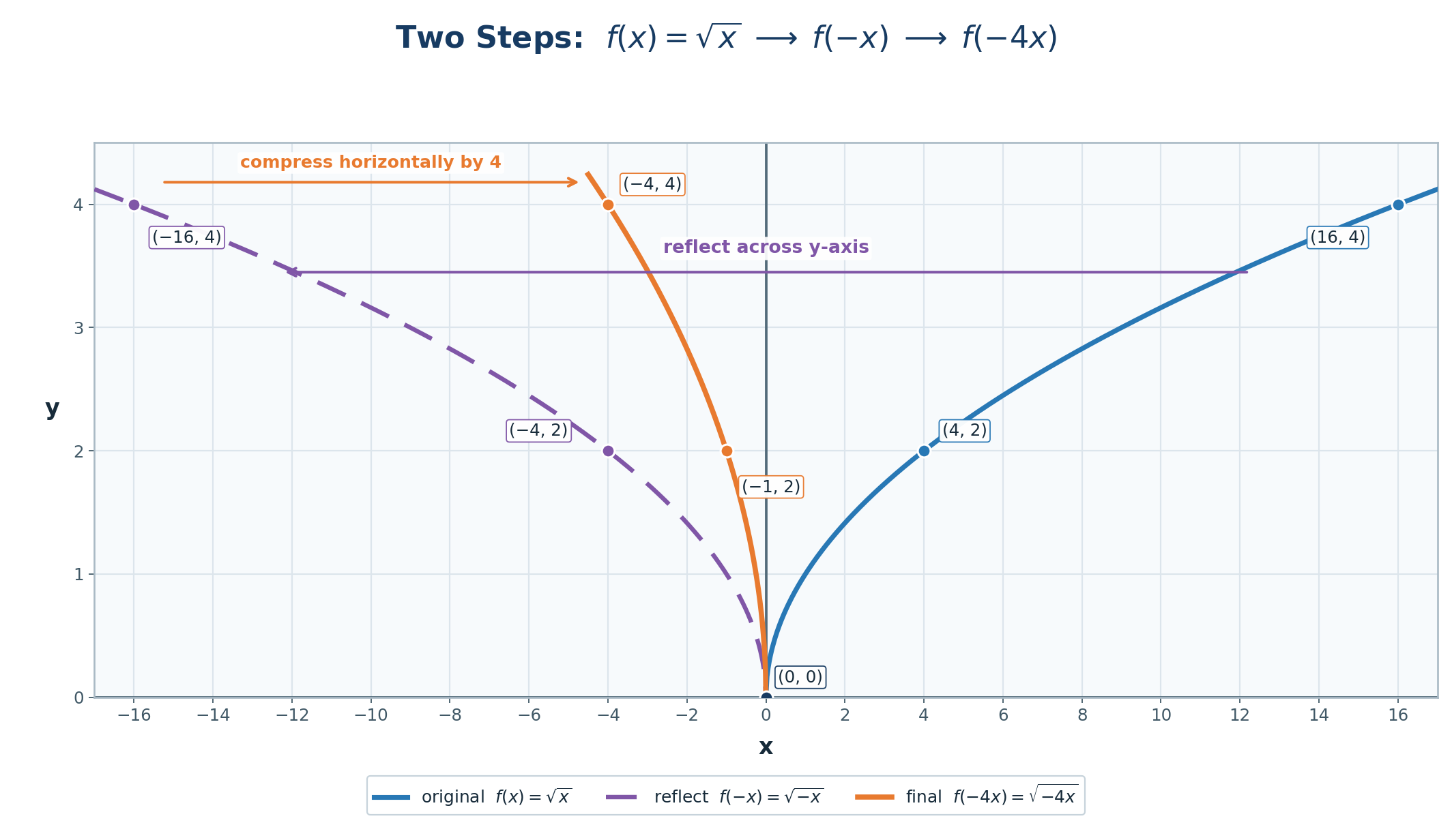
Let's trace f(x)=x under k=−4, giving g(x)=−4x.
Original
After reflecting
After squeezing by 4
(0,0)
(0,0)
(0,0)
(4,2)
(−4,2)
(−1,2)
(16,4)
(−16,4)
(−4,4)
The curve now lives to the left of the y-axis and reaches each corresponding height at one-fourth of the original horizontal distance from the y-axis. Notice that the domain flipped along with it: x accepts x≥0, while −4x accepts x≤0. The case k=−1 is simply the one where the magnitude is 1 — a pure mirror image with no change in width.
Try reflecting f(x)=x2 across the y-axis and something curious happens:
f(−x)=(−x)2=x2=f(x)
The new function is identical to the old one, so the graph does not appear to change at all. The same holds for f(x)=∣x∣, since ∣−x∣=∣x∣.
These graphs are already symmetric about the y-axis, meaning the left half is the mirror image of the right half, so mirroring them produces nothing new. Functions with this property are called even.
Asymmetric parents behave very differently. Reflecting x carries the whole curve to the other side of the plane, and reflecting f(x)=x turns the line y=x into y=−x. So when we want to test a claim about f(−x), it pays to pick a parent that is not symmetric, because a symmetric one hides the effect completely.
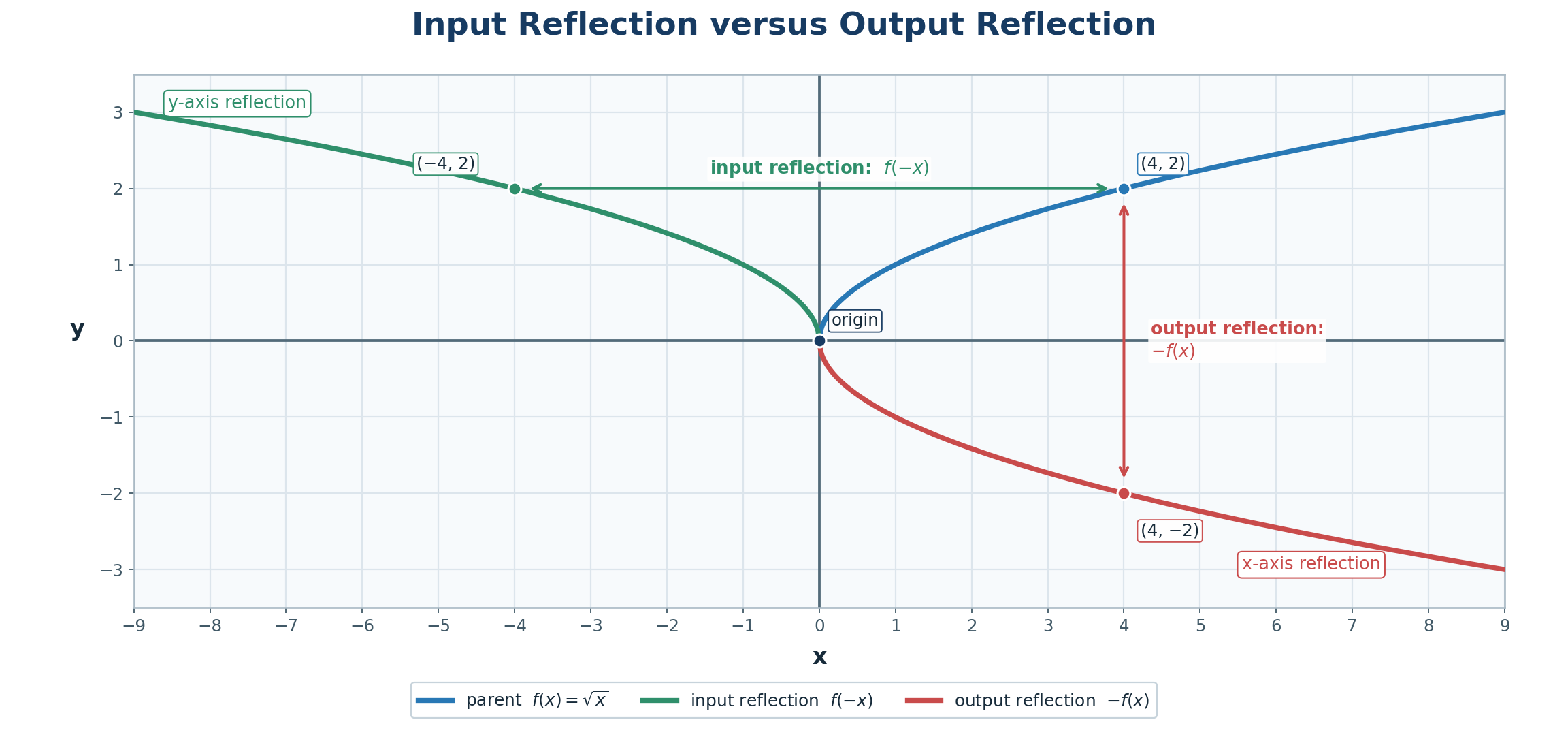
These two expressions look almost the same on the page and behave completely differently on the graph. Take f(x)=x and compare them point by point:
f(−x)=−x mirrors across the y-axis: heights stay positive, inputs turn negative, and the curve sits above the axis on the left side.
−f(x)=−x mirrors across the x-axis: inputs stay positive, heights turn negative, and the curve hangs below the axis on the right side.
A single point settles the difference. Under the input reflection, (4,2) becomes (−4,2); under the output reflection, it becomes (4,−2). The contrast is clearest with all three curves on the same axes.
Going the other way — from a picture back to k — takes the same two questions we used for output scaling, only aimed sideways. First, does an identifiable left-right feature move to the mirror side? If the parent is not symmetric about the y-axis and it does, then k is negative. For a graph symmetric about the y-axis, such as x2 or ∣x∣, the reflection is hidden, so the sign can be recovered only from identified corresponding points or the rule itself. Second, is it narrower or wider? Compare one convenient point's distance from the y-axis: if that distance was cut in half, the magnitude is 2; if it doubled, the magnitude is 21.
Here is a compact summary worth keeping nearby.
Factor k
Effect on the graph
Example point (6,y) becomes
k>1
Horizontal compression toward the y-axis
k=3: (2,y)
0<k<1
Horizontal stretch away from the y-axis
k=21: (12,y)
k=−1
Reflection across the y-axis
(−6,y)
k<−1
Reflection plus compression
k=−3: (−2,y)
−1<k<0
Reflection plus stretch
k=−21: (−12,y)
When a matched pair of points is available, one division does the whole job: k=xold/xnew, using any point with xnew=0. Both the sign and the magnitude drop out of that single quotient.
Input scaling mirrors output scaling in nearly every respect. Multiplying inputs by k maps (x,y) to (x/k,y), squeezing the graph toward the y-axis when ∣k∣>1, widening it away from the y-axis when ∣k∣<1, and reflecting it across the y-axis when k is negative. Heights never change, the y-intercept holds its ground, and the whole reciprocal effect traces back to one small equation: to reproduce a familiar output, the new input must satisfy kx=xold.
Now let's make it concrete. In the exercises ahead, we will adjust a factor and watch the graph respond, map points in both directions, complete the algebraic argument for the reversal, spot which parents survive a y-axis reflection untouched, and sketch f(−x), −f(x), and f(−2x) side by side. That last comparison is the real test of whether the two reflections stay separate in our minds, and the work in this lesson has us ready for it.