Welcome back to Stretching, Squeezing, and Reflecting Graphs! This is the third and final lesson of the course, and it is the one where the two scalings we studied separately are finally placed side by side and told apart.
Up to now, every problem told us where the factor lived. Lesson 1 handed us kf(x) and we scaled the outputs; Lesson 2 handed us f(kx) and we scaled the inputs. Out in the wild, transformations do not come labeled. What we usually get is a before and an after — two graphs, or two columns in a table — and the question "what happened here?"
So today we do detective work. We will pin down the clues that reliably separate an output scaling from an input scaling, recover the factor from a single matched pair of points, and then run a scaling and a shift together in the order the notation demands, because the other order lands us on a different graph entirely.
One Picture, Two Possible Causes
Picture two snapshots of the same curve, taken before and after some transformation. The new curve is taller and narrower than the old one. Two completely different stories explain that picture equally well: the outputs were multiplied by something bigger than 1, or the inputs were, pulling everything toward the y-axis.
This is the same ambiguity a business analyst faces when a revenue chart looks "bigger." Did every day earn twice as much, or did the same pattern of earnings simply play out in half the time? Those are very different events that can produce a similar-looking spike.
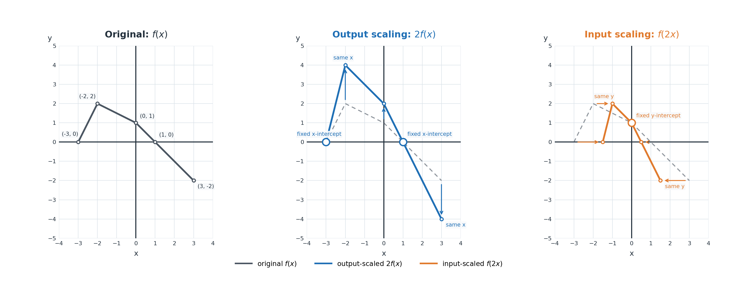
The way out is to stop judging the overall shape and start tracking individual points and the direction they traveled. Output scaling moves every point straight up or down, since (x,y)→(x,ky) never touches the first coordinate. Input scaling moves every point straight left or right, since (x,y)→(x/k,y) never touches the second. One transformation is pure vertical motion, the other pure horizontal motion, and that distinction survives even when the silhouettes look alike.
The Fixed Points Give It Away
Some points refuse to move at all, and identifying them is our single most reliable piece of evidence. As we saw in Lesson 1, multiplying outputs cannot budge a point whose height is already zero, because k⋅0=0. As we saw in Lesson 2, multiplying inputs cannot budge a point sitting at x=0, because 0/k=0.
That gives us two clean signatures to test against any before-and-after pair.
What stayed fixed
What it suggests
The x-intercepts (points on the x-axis)
Possible output scaling: g(x)=kf(x); verify with a matched non-axis point.
The y-intercept (the point on the y-axis)
Possible input scaling: g(x)=f(kx); verify with a matched non-axis point.
Fixed points are useful clues, not conclusive proof: output scaling can also preserve the y-intercept when f(0)=0, and input scaling can preserve an x-intercept at the origin. Confirm the diagnosis with a matched non-axis point: output scaling keeps its x-coordinate and changes y, whereas input scaling keeps y and changes x.
Join the 1M+ learners on CodeSignal
Be a part of our community of 1M+ users who develop and demonstrate their skills on CodeSignal
Tables sharpen the same evidence, because we can compare columns directly instead of eyeballing distances. Below is a mystery function f sampled at four points and transformed in two different ways.
Original point on f
Version A
Version B
(−2,4)
(−2,8)
(−1,4)
(0,−2)
(0,−4)
(0,−2)
(1,0)
(1,0)
(0.5,0)
(3,4)
(3,8)
(1.5,4)
In Version A the inputs are untouched and every height has doubled, including the y-intercept, which dropped from −2 to −4. The zero at x=1 did not move. That is an output scaling: A(x)=2f(x).
In Version B the heights match the original exactly and only the inputs changed, each one halved. The y-intercept held its value of −2, while the zero slid from x=1 to x=0.5. That is an input scaling, and one division recovers the factor: k=1/0.5=2, so B(x)=f(2x). Both recovery formulas are worth memorizing together:
koutput=yoldynew,kinput=xnewxold
Use a matched point where yold=0 to recover an output factor, or where xnew=0 to recover an input factor.
Honesty requires one caution before we trust this method everywhere. For the simplest parent graphs, the two scalings can produce exactly the same curve, and no amount of staring will separate them. Watch f(x)=x2 under an input factor of 2:
f(2x)=(2x)2=4x2=4f(x)
Squeezing this parabola horizontally by 2 is indistinguishable from stretching it vertically by 4. The same coincidence appears with f(x)=x, with f(x)=∣x∣, and with f(x)=x, where 4x=2x.
This is exactly why good diagnostic questions use graphs with more personality: a curve that is not symmetric, whose y-intercept sits away from the origin, or that carries a distinctive corner or endpoint. On such a graph the fixed points tell one unambiguous story, and that is the kind of evidence we will be asked to cite.
Diagnosis handled, let's turn to construction: performing two transformations in sequence. The form we will work with is
g(x)=kf(x)+c
and its point rule follows the arithmetic literally — take the original height, multiply by k, then add c:
(x,y)→(x,ky)→(x,ky+c)
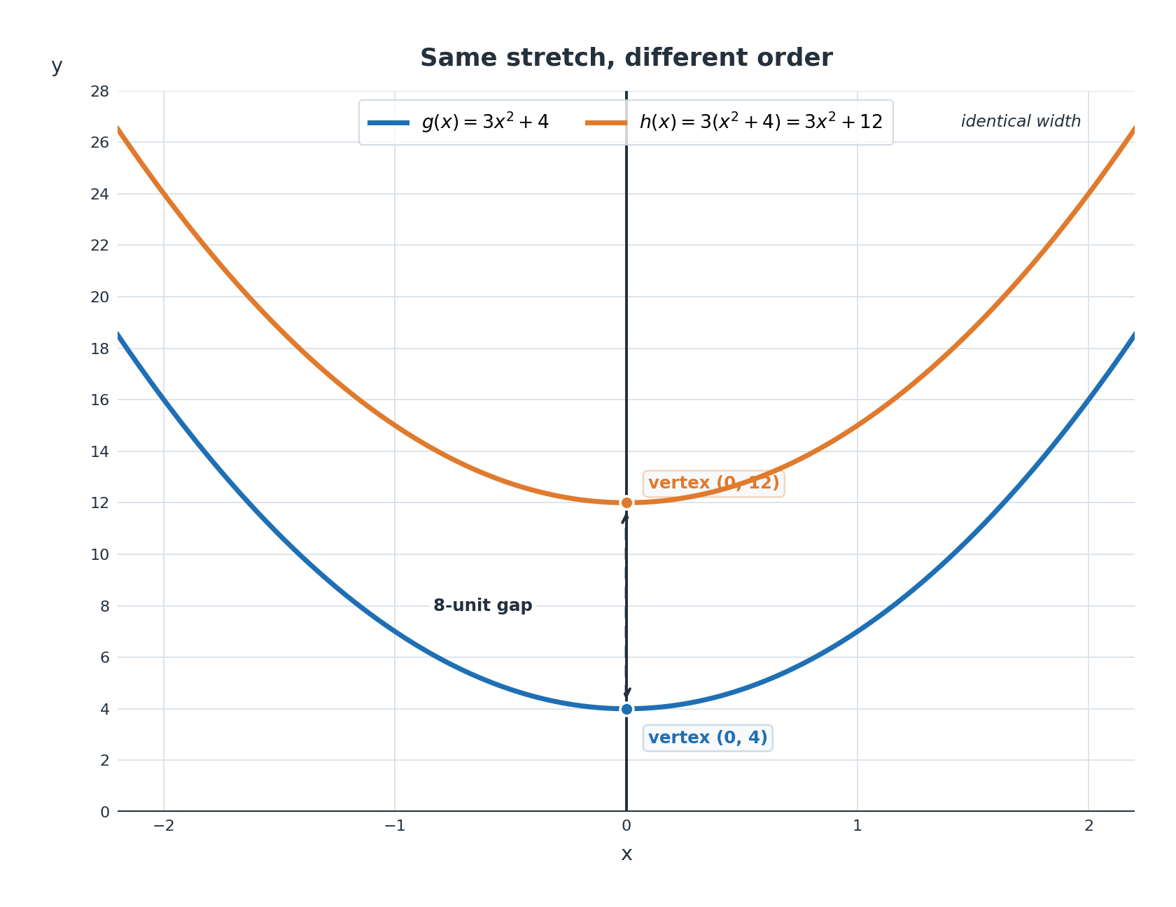
Let's run f(x)=x2 with k=3 and c=4, so g(x)=3x2+4. Walking the vertex and two reference points through both stages keeps the operations from blurring together.
Original
After stretching by 3
After shifting up 4
(0,0)
(0,0)
(0,4)
(1,1)
(1,3)
(1,7)
(2,4)
(2,12)
(2,16)
Notice that the shift is applied to the already stretched heights, never to the original ones. Writing the two stages in separate columns costs a few seconds and prevents most of the mistakes people make here.
So what if we shift first and stretch afterward? That is a genuinely different function, and the notation announces it:
h(x)=3(f(x)+4)=3x2+12
The vertex now travels (0,0)→(0,4)→(0,12), ending eight units above where g placed it. Both graphs are parabolas stretched by the same factor of 3, so their shape and width are identical, but they sit at different heights. The shift got multiplied along with everything else, which is why the gap is 3⋅4−4=8.
Shoppers meet this every day. A store offering 20% off and a $10 coupon can compute 0.8x−10 or 0.8(x−10), and on a $100 cart those come to $70 and $72. Same ingredients, different order, different total — which is why receipts spell out the sequence.
kf(x)+c=k(f(x)+c)whenever k=1 and c=0
Reading the order off the page is just ordinary arithmetic precedence. In kf(x)+c, the multiplication binds first, so we stretch, then shift. In k(f(x)+c), the parentheses force the addition first, so we shift, then stretch.
Negative factors deserve one careful pass, because the reflection and the shift are the easiest pair to swap by accident. Take f(x)=x with k=−2 and c=1, giving g(x)=−2x+1. We handle it in the same two stages, reading −2 as a reflection across the x-axis combined with a vertical stretch by 2.
Original
After scaling by −2
After shifting up 1
(0,0)
(0,0)
(0,1)
(1,1)
(1,−2)
(1,−1)
(4,2)
(4,−4)
(4,−3)
(9,3)
(9,−6)
(9,−5)
The curve flips to hang below its endpoint and falls twice as fast, and only then does the whole thing rise by one unit. The common slip is to shift the endpoint up first and reflect afterward, which would send (0,0) to (0,1) and then to (0,−1) — a different graph with a different endpoint. The written form −2x+1 tells us plainly that the multiplication comes first.
We now have a full toolkit for scalings. To diagnose one, we ask which points refused to move: fixed x-intercepts and unchanged inputs point to kf(x), while a fixed y-intercept and unchanged heights point to f(kx). To measure the factor, we divide a matched pair, ynew/yold for outputs or xold/xnew for inputs. And to combine a scaling with a shift, we follow the order the notation prescribes, scaling before adding in kf(x)+c and remembering that the reverse order produces a genuinely different graph.
The exercises ahead are where this becomes second nature. We will judge before-and-after pairs on sight, match clues to their signatures, walk anchor points through both stages of combined forms including a negative factor, plot two orderings of the same ingredients and watch them separate on screen, and finally write a full diagnosis defended with specific points. Let's go earn that evidence.