Welcome to Stretching, Squeezing, and Reflecting Graphs! This is the first lesson of the course, and it opens a genuinely new chapter in our work with graph transformations.
So far, we have moved graphs around without changing their shape. Adding a constant to the outputs slid a graph up or down, and subtracting a constant inside the function slid it left or right. Every point traveled the same distance in the same direction, so the curve kept its exact size and form.
Now we change the operation. Instead of adding to the outputs, we will multiply them, and multiplication does something translations never could: it changes how tall the graph is, and, when the factor is negative, it flips the graph upside down. By the end of this lesson, we will be able to predict and sketch k⋅f(x) for any factor, whether it is large, small, or negative.
Why Multiplying Outputs Changes Height
Picture a graph as a set of measurements taken over time, say the height of a bouncing ball recorded every tenth of a second. A translation is like re-measuring from a different floor level: every reading changes by the same amount. Multiplying is a different story entirely. It is like discovering that our ruler was marked in half-units, so every reading has to be doubled.
Notice what that correction does to the numbers. A reading of 4 becomes 8, a reading of 1 becomes 2, and a reading of 0 becomes... still 0.
Small values change a little, large values change a lot, and zero does not change at all. That single observation is the heart of this entire lesson.
The Mapping (x, y) → (x, ky)
As you may recall from earlier work, the cleanest way to describe a transformation is to say where each point goes. For the new function g(x)=k⋅f(x), the rule is:
(x,y)→(x,ky)
The x-coordinate is copied over untouched, and that is not a quirk of notation — it follows from where k sits in the formula. To compute k⋅f(x) at some input, we first hand that input to f exactly as it is, collect an output, and only then multiply. The input never meets k, so it never changes.
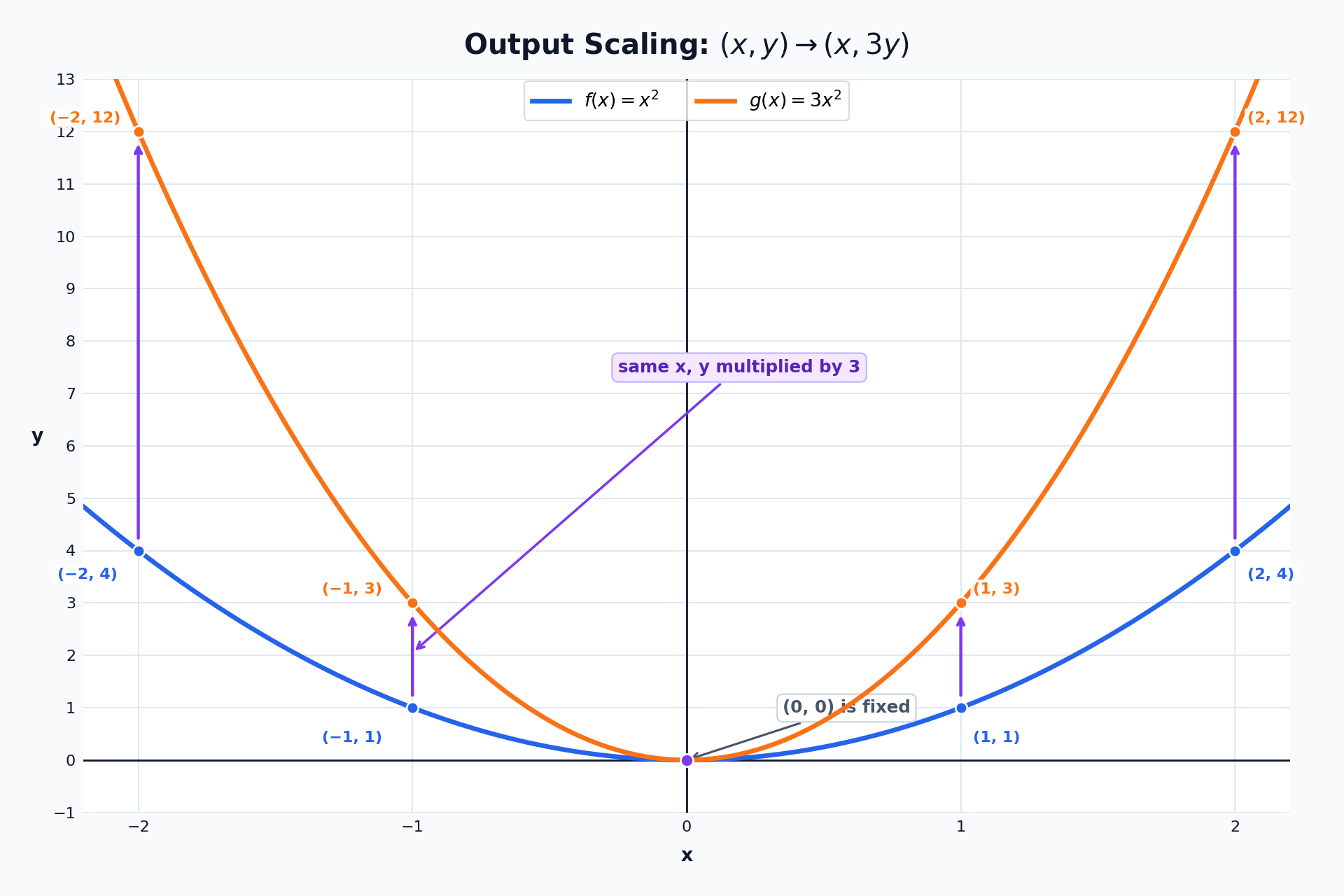
Let's apply the rule to f(x)=x2 with k=3, which gives g(x)=3x2.
x
f(x)=x2
g(x)=3x2
Point moves
−2
4
12
(−2,4)→(−2,12)
−1
1
3
(−1,1)→(−1,3)
0
0
0
(0,0)→(0,0)
1
1
3
(1,1)→(1,3)
2
4
12
(2,4)→(2,12)
Every point stays in its own vertical column and simply gets pulled to three times its original height.
Join the 1M+ learners on CodeSignal
Be a part of our community of 1M+ users who develop and demonstrate their skills on CodeSignal
Factors Greater Than One: Vertical Stretch
Factors Between Zero and One: Vertical Compression
When k>1, every output grows in magnitude, so the graph is stretched vertically. It looks taller and, in the case of a parabola, visually narrower.
That word narrower deserves care. The graph of y=3x2 certainly looks thin, but nothing was squeezed sideways. The point (2,4) did not slide toward the y-axis; it rose straight up to (2,12).
The curve only appears narrow because it reaches any given height sooner than the original did. We will come back to this at the end of the lesson, since it is the most common misconception about scaling.
When 0<k<1, every output shrinks toward zero, so the graph is compressed vertically. It looks flatter and wider, though once again nothing actually moved horizontally.
Take f(x)=∣x∣ with k=21, giving g(x)=21∣x∣:
(−4,4)→(−4,2)
(−1,1)→(−1,21)
(0,0)→(0,0)
(4,4)→(4,2)
The V-shape keeps its vertex at the origin and still opens upward, but its arms rise half as fast. Here is a real-world reading of the same idea: if f tracks a company's monthly revenue, then 21f tracks a branch that performs at half the rate — the busy and slow months land on exactly the same dates, only the amounts shrink.
Look back at both examples, and notice that the point (0,0) stayed exactly where it was each time. The reason is a single line of arithmetic, and it holds for every factor k:
k⋅0=0
If f(a)=0, then k⋅f(a)=0 as well, so the point (a,0) maps to itself. Points on the x-axis are the fixed points of any output scaling, and the x-axis itself acts as the line that the graph is stretched away from or squeezed toward, much like a rubber sheet pinned along that line.
This hands us a fast diagnostic. If a graph has been scaled through its outputs, its x-intercepts must be exactly where they were before.
A negative factor may look like a brand-new case, but it is really two familiar steps combined. We simply split k into its sign and its magnitude:
k⋅f(x)=(−1)⋅(∣k∣⋅f(x))
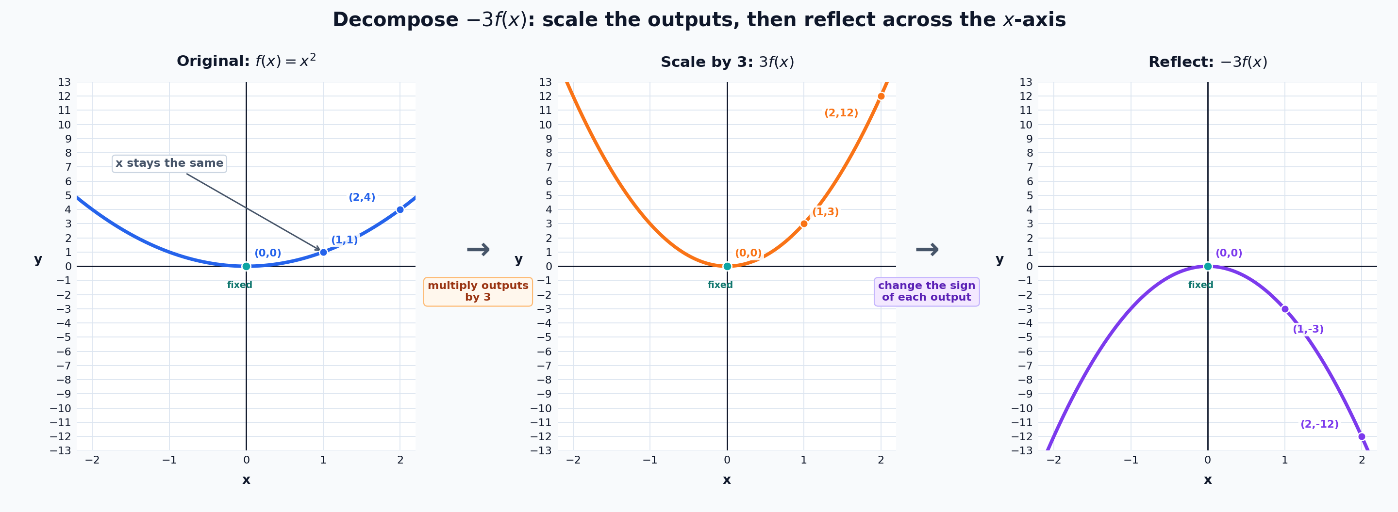
So working with k=−3 means scaling by the magnitude 3, which triples every y-value, and then reflecting across the x-axis, which flips the sign of every y-value. Multiplying by −1 sends (x,y) to (x,−y), placing each point the same distance from the x-axis but on the opposite side — precisely a reflection. The order of the two steps does not matter, since multiplication can be carried out in either order.
Let's trace f(x)=x2 under k=−3:
Original
After scaling by 3
After reflecting
(1,1)
(1,3)
(1,−3)
(2,4)
(2,12)
(2,−12)
(0,0)
(0,0)
(0,0)
The parabola now opens downward and is three times as tall in the downward direction. And notice that k=−1 is just the special case where the magnitude equals 1: a pure reflection with no change in size at all.
Going the other direction — from a picture back to the number k — takes two questions, and it works best to ask them together rather than one at a time. First, is the graph flipped? If the curve opens the opposite way, or every output has switched sign, then k is negative. Second, is it taller or flatter? Compare one convenient point's distance from the x-axis: if that distance doubled, the magnitude is 2; if it halved, the magnitude is 21.
Here is a compact summary worth keeping nearby:
Factor k
Effect
Example point (2,4) becomes
k>1
Vertical stretch
k=2: (2,8)
0<k<1
Vertical compression
k=41: (2,1)
k=−1
Reflection across the x-axis
(2,−4)
k<−1
Reflection plus stretch
k=−2: (2,−8)
−1<k<0
Reflection plus compression
k=−21: (2,−2)
When we can read off a matched pair of points, there is an even faster route: divide the new output by the old one, k=yoldynew, using any point where yold=0. The sign and the magnitude both fall out of that one division.
The hardest case to picture is a negative factor with a fractional magnitude, such as g(x)=−21x. Decomposing it removes all the guesswork: start with x, halve every output, then flip across the x-axis. The point (4,2) becomes (4,1) and then (4,−1), while the endpoint (0,0) stays exactly where it began.
Now the warning that gives this section its name. Learners often describe a stretched graph as "squeezed from the sides" and a compressed graph as "stretched sideways," and neither description is true for k⋅f(x).
The reason is the mapping itself: x-coordinates are never touched. The domain is unchanged, every x-intercept is unchanged, and each point travels along a strictly vertical path. Whenever the picture feels ambiguous, pick one specific point and track it — the x-coordinate will settle the argument.
We have added a genuinely new tool to our collection. Multiplying outputs by k maps (x,y) to (x,ky), which stretches the graph when ∣k∣>1, compresses it when ∣k∣<1, and reflects it across the x-axis when k is negative. Any negative factor splits cleanly into a reflection and a scaling of magnitude ∣k∣, and through all of it, the inputs stay put and the x-intercepts hold their ground.
Time to put this into action. In the exercises ahead, we will move points under a given factor, split negative factors into their two steps, match graphs to their scalings, and read a signed factor straight off a curve. Keep the mapping (x,y)→(x,ky) in mind, and every one of those tasks becomes a matter of careful arithmetic rather than guesswork.