Right and Left Skew
Introduction
Welcome back to Skewed Distributions! In the previous lesson we learned to spot asymmetric shapes with one long tail and tell them apart from the symmetric bell and the flat uniform. That was the first step, and now we are ready for the second: naming the direction of the skew correctly.
This lesson focuses on the distinction between right skew and left skew. We will learn a simple naming rule, see it applied to familiar examples, and tackle a surprisingly common mix-up that trips up even experienced readers of data. By the end, we will be able to look at any skewed distribution and confidently call it by the right name.
The Tail Tells the Name
We already know that a skewed distribution has two visually distinct sides: one where the data piles up steeply, and one where a thinner tail stretches out. The natural follow-up question is: how do we describe which way the skew goes?
The answer is refreshingly simple. We name a skewed distribution by the direction its long tail points, not by where the bulk of the data sits. The tail is the narrator — it tells us the name. Let's see this rule in action with both directions.
Right Skew
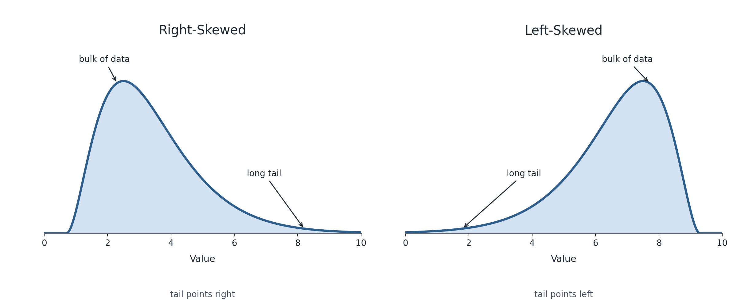
A distribution is called right-skewed (or positively skewed) when its long tail extends toward the right side of the number line — that is, toward higher values. In this shape, most observations cluster on the left near smaller values, and a thin trail of uncommon, larger values stretches to the right.
Picture a histogram of restaurant meal prices at a casual dining chain. Most meals cost somewhere between $10 and $20, creating a tall cluster on the left. But a few premium specials push prices to $40 or beyond, pulling a long tail to the right. Because the tail points right, we call this distribution right-skewed.
The alternate name positively skewed comes from the number line: the tail reaches toward the positive (larger) end. Both names mean exactly the same thing.
Left Skew
A distribution is called left-skewed (or negatively skewed) when its long tail extends toward the left side of the number line — toward lower values. Here, most observations gather on the right near higher values, while a thinner trail of unusually low values stretches to the left.
Think about exam scores on a test that most students found fairly easy. The bulk of scores pile up near 85–100, forming a peak on the right. A handful of students scored much lower, pulling a tail toward the left. Because the tail points left, we call this distribution left-skewed.
Just as before, the alternate name negatively skewed reflects the fact that the tail reaches toward the lower (more negative) end of the number line.
Side-by-Side Comparison
Placing the two shapes next to each other makes the contrast unmistakable.
| Feature | Right-Skewed | Left-Skewed |
|---|---|---|
| Long tail points | Right (toward higher values) | Left (toward lower values) |
| Bulk of data sits | On the left (lower values) | On the right (higher values) |
| Peak is closer to | The left end | The right end |
| Also called | Positively skewed | Negatively skewed |
Notice a pattern in the table: the tail and the bulk are always on opposite sides. This is precisely what creates the asymmetry we identified in our first lesson. The naming rule always follows the tail, never the bulk.
The Most Common Mix-Up
Here is where many learners stumble, so let's address it head-on. When we glance at a skewed distribution, the bulky side is visually dominant — it takes up most of the graph. It is tempting to say, "Most of the data is on the left, so this must be left-skewed." That reasoning feels natural, but it leads to the wrong name every single time.
The fix is a short mental check we can use whenever we need to label a skew:
- Find the long tail — the side that stretches out thinly.
- Ask: Does that tail point to the right or to the left?
- That direction is the name of the skew.
If the bulk sits on the left and the tail reaches right, the distribution is right-skewed, not left-skewed. If the bulk sits on the right and the tail reaches left, it is left-skewed, not right-skewed. Always follow the tail.
A Quick Mental Shortcut
One handy way to lock in the naming rule is to imagine the distribution as an animal with a tail. The animal's body is the bulk of the data, and the tail sticks out on the opposite side. We name the skew by where the tail points, just as we might say "the cat's tail is pointing to the right." The body faces the other direction, but that is not what we use for the name.
This small image can save us from the bulk-versus-tail confusion in the heat of the moment, especially when a graph appears without labels and we need to make a quick call. Whenever in doubt, look past the big bulky hump and focus on the thin, stretched-out side — that side gives the distribution its name.
Conclusion and Next Steps
In this lesson we learned that skew is named for the direction of the long tail, not for where the majority of the data clusters. A right-skewed distribution has its tail extending toward higher values on the right, while a left-skewed distribution has its tail reaching toward lower values on the left. We also confronted the most common naming mistake and practiced a simple three-step check: find the tail, note its direction, and use that direction as the name.
Coming up next, you will put this naming convention to work in a set of practice exercises. You will identify tail directions, complete statements about the naming rule, label tricky shapes where the bulk and tail sit on opposite sides, and write your own justification for a real-world example. Let's see how sharp that tail-spotting skill has become!
