Explaining Right Skew
Introduction
Welcome back to Skewed Distributions! This is lesson three of four, so we are well past the halfway mark. In the first two lessons we built a toolkit for seeing and naming skewed shapes: we learned to spot asymmetry with one long tail and to label the skew by the direction that tail points. Now comes the deeper question — what makes a distribution skewed in the first place?
In this lesson we focus on right skew and the surprisingly simple mechanism behind it. We will see why variables like household income, home prices, and customer wait times almost always lean the same way. Once the mechanism clicks, we will be able to predict right skew before we even look at a graph.
From Describing to Explaining
Recognizing a shape and explaining its cause are two very different skills. If someone shows us a histogram of home sale prices and asks, "Is this right-skewed?" we can answer by finding the long tail. But if a colleague mentions a variable we have never plotted — say, the time customers spend on hold with a support line — and asks, "What shape would you expect?" we need a reason, not just a visual memory.
That reason comes from understanding the process that generates the data. When we know what kind of process tends to create right skew, we can apply that logic to any new variable and make a well-founded prediction. The rest of this lesson builds that reasoning, one ingredient at a time.
A Natural Floor
Many everyday quantities share a quiet but important feature: they cannot drop below some low value. This lower boundary is often called a floor. Here are a few familiar examples:
- Household income is often treated as having a floor near $0 for this kind of example.
- Home sale prices cannot be negative — a house sells for at least some positive amount.
- Wait time on a support line starts at zero; no one waits a negative number of minutes.
- Reaction time has a biological minimum around 150–200 milliseconds; our nervous system simply cannot fire faster.
A floor squeezes the left side of the distribution. Values cannot spread out very far in that direction because the boundary stops them. Think of it like a wall on the left: data can pile up against it, but it cannot pass through.
Room to Stretch on the Right
Now look at the other side. While a floor blocks values from going much lower, there is usually no matching ceiling on the upper end. Nothing in the rules of economics caps how high a single household's income can climb. Nothing stops a luxury home from listing at many times the typical price. And every now and then, a customer on a support line waits far longer than most.
These uncommon but perfectly real observations sit far above the bulk, pulling the right tail outward. The key word here is occasional: most values stay near the floor, but a few stretch far to the right. With no hard upper boundary to rein them in, those rare high values have unlimited room to roam.
The Recipe for Right Skew
We can now state the pattern cleanly. Right skew tends to appear whenever two ingredients come together:
- A floor near a low value that prevents data from spreading to the left.
- Occasional large values with no hard ceiling to stop them, stretching the distribution to the right.
The floor keeps the left side compact, while the rare high values pull the right tail long. That combination is exactly the asymmetry we see in a right-skewed shape.
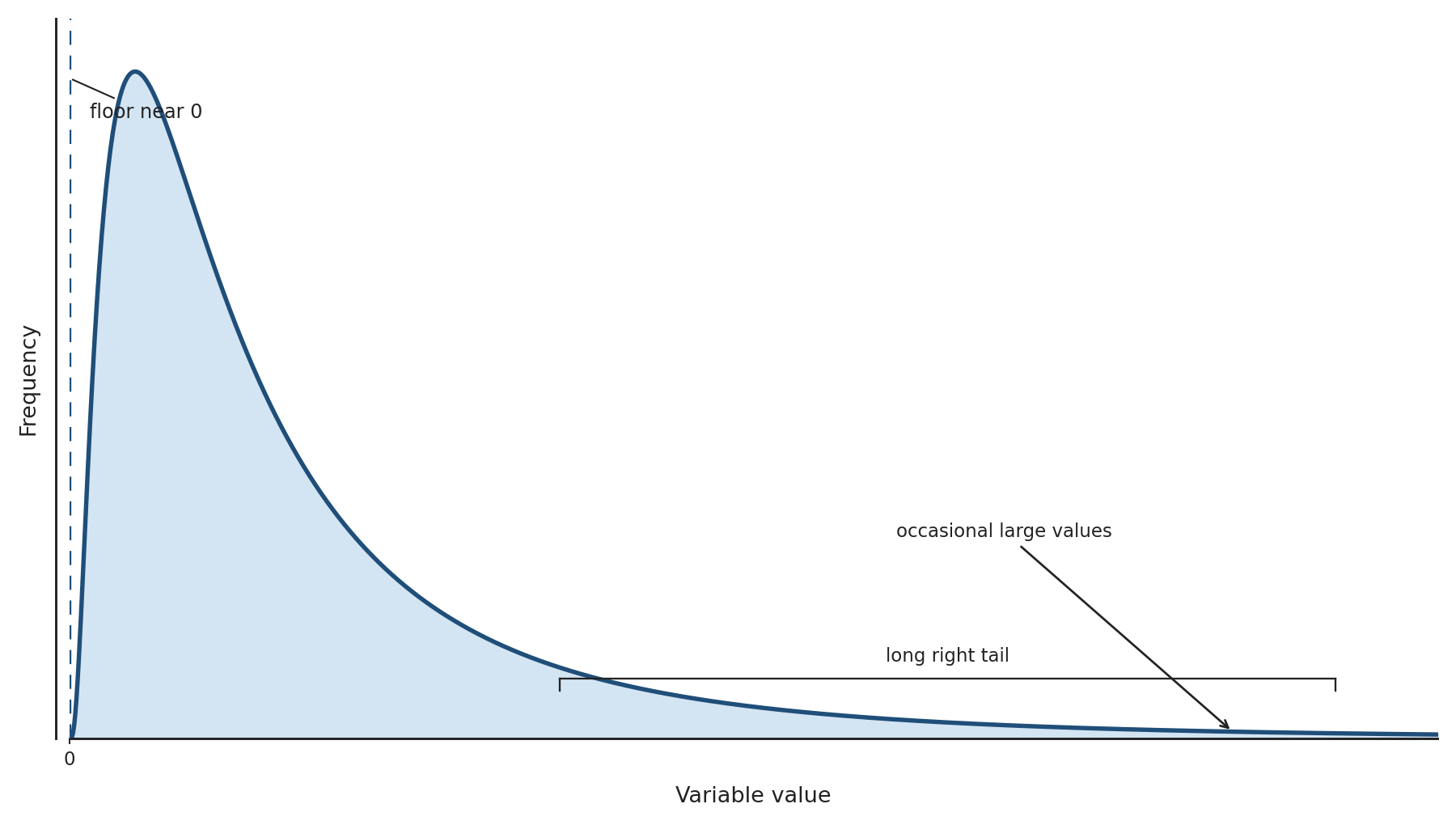
Whenever we spot both ingredients in a real-world variable, we have a strong reason to expect right skew — even before looking at a single graph. The recipe gives us predictive power, not just descriptive vocabulary.
The Recipe in Action
Let's apply the two-ingredient check to several well-known variables and confirm that both pieces are present every time.
| Variable | Where is the floor? | What creates occasional large values? |
|---|---|---|
| Household income | Near $0 | A small share of earners make very high salaries |
| Home sale prices | Must be positive; most cluster around a regional average | A few luxury or waterfront properties sell for many times the typical price |
| Call-center hold time | Zero minutes (instant pickup) | Some callers wait through long queues during peak hours |
| Reaction time | Biological minimum ~150–200 ms | Occasional slow responses due to distraction or fatigue |
In every row, the same story repeats: a floor compresses the left side and a handful of high values stretch the right tail. The process is the explanation; the shape is the result.
A Closer Look at Income
Household income is perhaps the most frequently cited example of right skew, so it deserves a closer look. Most households earn somewhere in a moderate range set by common wages and salaries. The floor is effectively near zero because income cannot be negative in most practical contexts. At the same time, there is no real upper limit — business owners, executives, and top professionals can earn many multiples of the median, and their incomes land far out in the right tail.
Notice that the right skew is not caused by one unusual person. It results from the process itself: a low-end boundary combined with an open-ended upper range. Any variable whose generating process looks like this will tend to be right-skewed, regardless of the specific numbers involved. That is why the recipe works so broadly — it is about the structure of the process, not the particular data.
Conclusion and Next Steps
In this lesson we moved from simply naming right skew to understanding why it happens. The recipe has two ingredients: a floor near a low value that keeps the left side compact, and occasional large values with no hard ceiling that stretch the right tail. We saw this pattern at work in household income, home prices, call-center hold times, and reaction times.
Up next, you will put this reasoning to the test in a set of practice exercises. You will identify which variables are likely right-skewed, complete an explanation using the floor-plus-occasional-large-values logic, and write your own reasoning for a new scenario. Time to turn that understanding into confidence!
