Explaining Left Skew
Introduction
Welcome back to Skewed Distributions! This is the fourth and final lesson of the course, so we are about to wrap things up. In the previous lesson we uncovered the simple two-ingredient recipe behind right skew: a floor near a low value plus occasional large values that stretch the right tail. That recipe gave us the power to predict right skew from a process, not just recognize it on a graph.
Now we turn the lens in the opposite direction. In this lesson we explore left skew and the mechanism that produces it. As we will see, the logic is a satisfying mirror image of what we already know. By the end, we will be able to look at real-world variables like customer satisfaction ratings or age at retirement and explain why their distributions lean the way they do.
Flipping the Recipe
As you may recall from Lesson 2, a left-skewed distribution has most of its data bunched toward the high end, with a long tail stretching toward lower values. If right skew looks like a hill pressed against a wall on the left with a tail trailing off to the right, then left skew is the mirror image: a hill pressed against a wall on the right with a tail trailing to the left.
Right skew gets a lot of attention because many well-known variables — income, home prices, wait times — follow that pattern. Left skew is just as important but often less familiar, which makes it all the more valuable to understand. Since right skew came from a floor combined with occasional high values, a natural question arises: can we simply flip each ingredient to explain left skew? That is exactly where we are headed.
A Natural Ceiling
Many real-world variables bump up against an upper boundary, often called a ceiling. This ceiling prevents values from climbing any higher, no matter how hard they try. Here are a few everyday examples:
- Customer satisfaction ratings on a 1‑to‑5 or 1‑to‑10 scale cannot exceed the top score.
- Age at retirement has a practical ceiling because most people retire by their mid-to-late 60s, and very few work beyond their early 70s.
- Time to finish a quick task before a deadline cannot exceed the deadline itself; the clock stops when time runs out.
- Exam scores are capped at 100% (or whatever the maximum is).
A ceiling compresses the right side of the distribution. Values cannot spread upward past the boundary, so they pile up near it. Think of it as a wall on the right: data clusters against it but cannot push through.
Room to Stretch on the Left
Now look at the other side. While a ceiling blocks values from going higher, the low end is far enough from the bulk that occasional values can land well below the crowd. A customer who had a terrible experience can leave a rating far below the typical score. Someone who retires early for health or financial reasons might leave the workforce years or even decades before most peers. And a person who breezes through a quick survey might finish well ahead of anyone else.
Some of these variables do have a technical lower bound — a satisfaction scale bottoms out at , and an exam score cannot drop below . But that lower bound is far away from where the bulk of the data clusters near the ceiling. The important point is not whether a floor exists at all, but whether there is enough room below the bulk for occasional values to stretch a long tail to the left.
These low observations are occasional, not typical. Most values huddle near the ceiling. But the few that drop well below have plenty of room to do so, pulling the left tail outward and creating the characteristic left-skewed shape.
The Recipe for Left Skew
We can now state the pattern as a clean mirror of the right-skew recipe. Left skew tends to appear whenever two ingredients come together:
- A ceiling near a high value that prevents data from spreading to the right.
- Occasional low values far enough from the bulk to stretch the distribution to the left.
The ceiling keeps the right side compact, while the rare low values pull the left tail long. That combination is precisely the asymmetry we see in a left-skewed shape.
Notice how neatly this mirrors the right-skew recipe. We have simply swapped "floor" for "ceiling" and "occasional large values" for "occasional low values." The underlying logic is the same: one boundary compresses one side, while room on the other side lets rare values stretch a long tail.
The Recipe in Action
Let's walk through several real-world variables and check that both ingredients are present in each case.
| Variable | Where is the ceiling? | What creates occasional low values? |
|---|---|---|
| Customer satisfaction ratings | Maximum score on the scale (e.g., out of ) | A few unhappy customers leave ratings far below the majority |
| Age at retirement | A practical upper boundary in the late 60s or early 70s | Some individuals retire much earlier due to health, wealth, or career changes |
| Time to finish a quick checkout survey | The survey deadline or closing time | A few fast responders finish well ahead of the rest |
| Exam scores (easy exam) | is the highest possible score | A handful of students score much lower than the well-prepared majority |
In every row, the same story plays out: a ceiling bunches most values near the top, and a handful of low values pull the left tail outward. The process explains the shape.
A Closer Look at Satisfaction Ratings
Customer satisfaction ratings are one of the most common examples of left skew, so let's dig a bit deeper. Imagine a company asks every customer to rate their experience on a scale from to . Most customers have a routine, perfectly fine experience and give scores of , , or . The ceiling at means no one can rate higher, so the right side of the distribution is tightly packed.
But every so often, a customer has a genuinely bad experience — a lost order, a rude interaction, or a billing error. That customer might rate the experience a or a . These low ratings are uncommon, yet they land far from the bulk, pulling a tail to the left.
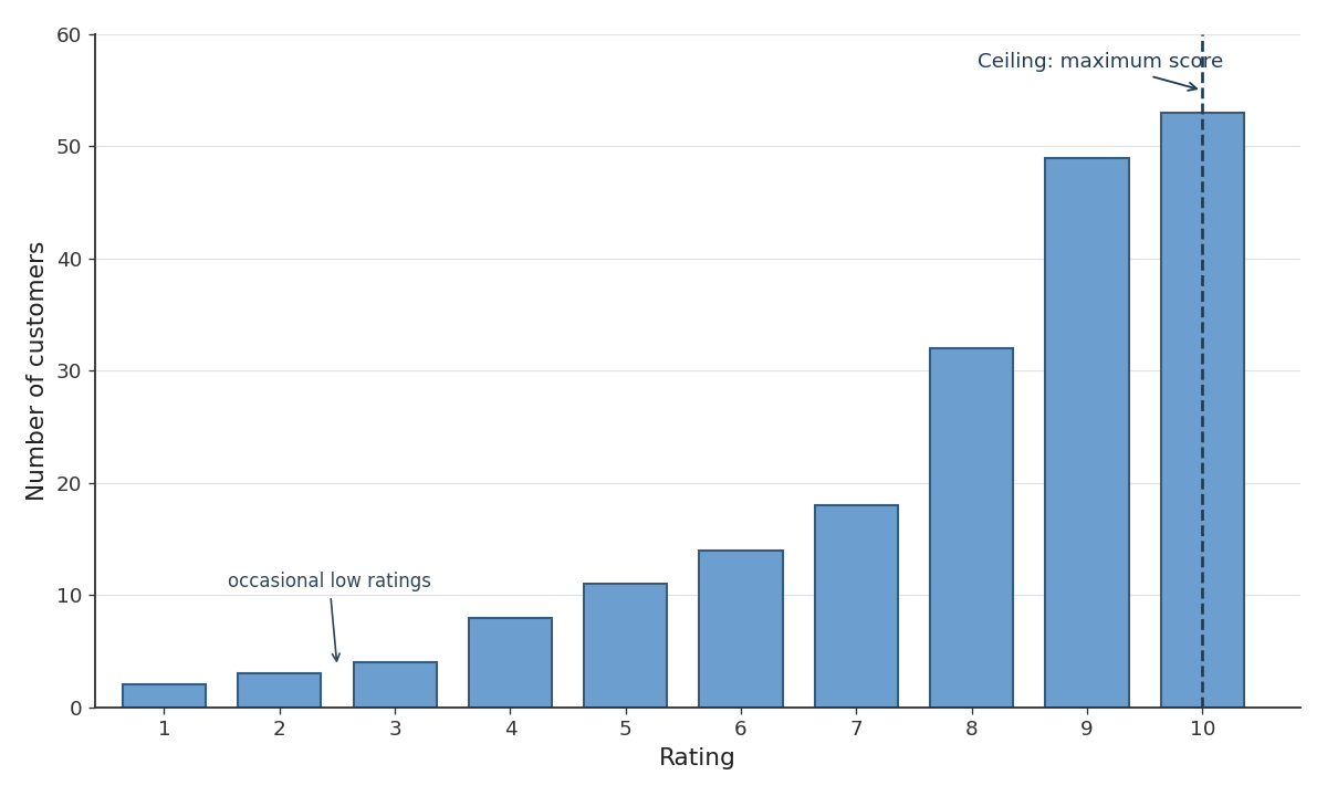
Notice the parallel to the income example we studied for right skew. There, a floor near zero and open-ended high earners created a right tail. Here, a ceiling at the top score and occasional low ratings create a left tail. The structure of the process is the explanation — and that structure is a perfect mirror image.
Conclusion and Next Steps
In this lesson we completed the picture by learning why left skew happens. The recipe has two ingredients: a ceiling near a high value that keeps the right side compact, and occasional low values that stretch the left tail. We saw this pattern in customer satisfaction ratings, age at retirement, quick-task completion times, and easy-exam scores.
Together with the right-skew recipe from the previous lesson, you now have a unified way to reason about skewed distributions: identify whether a process has a boundary on one side and room to stretch on the other, then name the skew by the direction of the long tail. Head into the exercises next, where you will spot left-skewed variables, explain the ceiling-plus-occasional-low-values logic, and build your own argument from scratch!
