What Skew Looks Like
Introduction
Welcome to Skewed Distributions, the fifth course in our learning path! Over the previous courses, we built a strong foundation: we learned to read distribution graphs, explored the flat uniform shape, studied the symmetric bell of the normal distribution, and counted successes with the binomial family. Now it is time to focus on distributions that break symmetry in a very recognizable way.
This first lesson is all about what skew looks like. By the end, we will be able to spot a skewed distribution at a glance and clearly tell it apart from the symmetric bell and the flat uniform shapes we already know.
Shapes We Have Seen So Far
Before we explore something new, let's briefly recall two important distribution shapes from earlier courses. The normal distribution forms a symmetric bell: a single peak sits in the center, and two tails trail off equally on both sides. The uniform distribution is flat, with every outcome roughly equally likely across the entire range.
Despite looking very different from each other, these two shapes share one key property: if we drew a vertical line down the middle, the left half would roughly mirror the right half. This mirror quality is what we call symmetry, and it is exactly the feature we are about to watch break.
When a Distribution Loses Its Balance
Imagine measuring household incomes in a large city. Most households earn somewhere in a moderate range, so we see a peak on the left side of the graph. But a small number of households earn far more than the rest, stretching the graph out to the right. The result is a shape that is clearly not symmetric: one side drops off quickly while the other side extends much farther.
This kind of lopsided shape is called a skewed distribution. The hallmark of skew is a single, noticeably longer tail on one side compared to the other. Where the bell curve tapers evenly in both directions and the uniform shape stays level, a skewed distribution tilts the weight to one side and lets a thin trail of uncommon values stretch away on the other.
The Defining Features of Skew
Two visual features set a skewed distribution apart from every other shape we have studied:
- Asymmetry — The shape is not a mirror image around its center. One side is compressed while the other is stretched out.
- One long tail — The bulk of the data clusters toward one end, and a thinner tail of less common values extends in the opposite direction.
Many skewed distributions look like a lopsided hill: the bulk is pushed toward one side, and a gentle slope trails off much farther on the other. Whenever we notice that contrast between a steep drop on one side and a gradual fade on the other, we are looking at skew.
Skewed vs. Symmetric vs. Flat
Now let's place all three shape families side by side so the differences are unmistakable.
![[Side-by-side comparison of normal, uniform, and skewed distribution shapes]](https://k3-production-bucket.s3.us-east-1.amazonaws.com/uploads/WTSacNdBzrYfrJheh_image.png)
| Feature | Normal (Bell) | Uniform (Flat) | Skewed |
|---|---|---|---|
| Symmetry | Symmetric | Symmetric | Asymmetric |
| Peak(s) | One peak in the center | No peak (flat top) | Often has a peak shifted toward one side |
| Tails | Two equal tails | No meaningful tails | One short tail, one long tail |
The quickest test for skew is to ask: Does one tail stretch noticeably farther than the other? If the answer is yes, the distribution is skewed. If both sides look like mirror images of each other, the shape is symmetric. And if the distribution is roughly level across all outcomes with no peak at all, it is uniform.
Spotting Skew in Everyday Data
Many real-world variables produce skewed shapes. Consider household water bills: most families use a similar amount of water each month, so the bills cluster around a typical value and create a peak. But a few households use much more — perhaps because of large gardens or swimming pools — pulling a tail of higher values out to one side.
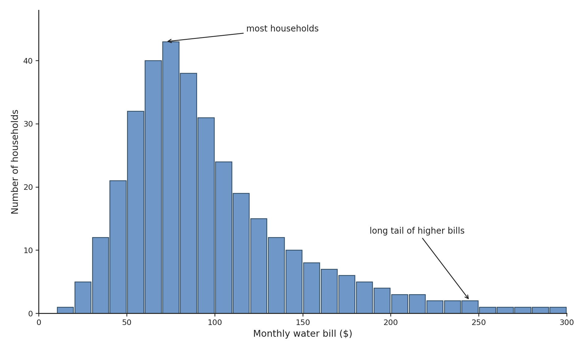
When we look at a graph like this, the giveaway is that one side fades out slowly while the other drops off quickly. The shape rises steeply, peaks early, and then trails off gradually — a textbook example of skew. No formulas are needed here; the shape alone tells the story.
Conclusion and Next Steps
In this lesson, we learned that a skewed distribution is an asymmetric shape with one noticeably longer tail. We contrasted it with the symmetric bell of the normal distribution and the flat line of the uniform distribution, and we saw that the fastest way to spot skew is to check whether one tail extends much farther than the other.
Up next is a set of hands-on practice exercises where you will identify skewed shapes among a lineup, match distribution families to their labels, and put your observations into words on a real-world example. Time to put that freshly trained eye to the test!
