Welcome to the first lesson of our course on realistic rendering techniques! If you've completed the foundational ray tracing course, you now have a working ray tracer that can render spheres with proper lighting and shading. However, if you look closely at the images your ray tracer produces, you'll notice something that makes them look less realistic: jagged edges, especially along the boundaries of objects.

These jagged edges are called "aliasing artifacts," and they're one of the most noticeable differences between a basic ray tracer and a production-quality renderer. When you render a sphere against a background, the edge where the sphere meets the sky appears as a staircase pattern rather than a smooth curve. Similarly, any diagonal lines or curved surfaces in your scene will have this harsh, pixelated appearance.

In this lesson, we'll explore why aliasing happens in the first place and, more importantly, how to fix it using a technique called antialiasing through random sampling. By the end of this lesson, you'll understand how to transform your ray tracer from producing images with harsh, jagged edges to generating smooth, professional-looking renders. The technique we'll learn is fundamental to all modern rendering systems, from movie production to video games.

To understand why we get jagged edges, we need to think about the fundamental mismatch between the continuous world we're trying to render and the discrete pixels we're rendering into. The real world is continuous — a sphere's edge is a perfectly smooth curve. But our digital image is made up of individual square pixels arranged in a grid, and each pixel can only be one color.

Let's consider a concrete example. Imagine a diagonal line passing through your image at a 45-degree angle. In the real world, this line is infinitely thin and perfectly straight. But when we try to represent it with pixels, we have to make a binary decision for each pixel: is this pixel part of the line or not? The result is a staircase pattern where the line jumps from one row of pixels to the next.

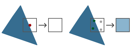
In our current ray tracer, we shoot exactly one ray per pixel, typically through the center of that pixel. This single ray determines the entire color of that pixel. If the ray hits the sphere, the pixel is colored based on the sphere's surface. If it misses, the pixel gets the background color. There's no middle ground, no blending — just a hard decision for each pixel.

This binary approach works fine in the middle of a surface where all nearby rays would give similar results. But at the edge of an object, adjacent pixels can have completely different colors. One pixel's ray might just barely hit the sphere and return a surface color, while the next pixel's ray might just barely miss and return the sky color. This creates the harsh, staircase-like boundary we see as aliasing.

The problem is most visible at high-contrast edges, like where a dark sphere meets a bright sky. The human eye is particularly sensitive to these sharp transitions, making the jagged pattern very noticeable. Even though each individual pixel is "correct" based on the single ray we shot through it, the overall image doesn't look smooth because we're missing information about what's happening between those sample points.

The solution to aliasing is conceptually straightforward: instead of shooting just one ray per pixel, we shoot multiple rays per pixel and average the results. This technique is called supersampling, and it's one of the most effective ways to improve image quality in ray tracing.

Here's the core idea: if we shoot multiple rays through different positions within a single pixel, we gather more information about what that pixel should look like. For a pixel right at the edge of a sphere, some of those rays might hit the sphere while others miss it. When we average all these samples together, we get a color that's somewhere between the sphere color and the background color — exactly what we need for a smooth edge.

Think of it like taking a survey. If you ask one person their opinion, you get a single answer that might not represent the full picture. But if you ask fifty people and average their responses, you get a much more reliable result. The same principle applies here: more samples give us more information, leading to better decisions about what color each pixel should be.

Let's say we're rendering a pixel that's half-covered by a sphere. With a single sample, we'd get either the sphere color or the sky color depending on where exactly that one ray went. But with fifty samples randomly distributed across the pixel, roughly twenty-five would hit the sphere and twenty-five would hit the sky. When we average these together, we get a color that's halfway between the two — a perfect representation of a pixel that's half-covered by the sphere.

The trade-off, of course, is computational cost. If we shoot fifty rays per pixel instead of one, our rendering takes roughly fifty times longer. This is why samples_per_pixel is a quality setting in most renderers: higher values produce smoother images but take more time. For quick previews, you might use just a few samples per pixel. For final production renders, you might use hundreds or even thousands.

Now that we understand the value of multiple samples per pixel, we need to decide where to place those samples within each pixel. You might think the logical approach would be to arrange them in a regular grid — for example, if we want four samples per pixel, we could place them in a 2×2 grid pattern. While this would work, there's a better approach: random sampling.

The key advantage of random sampling is how it handles errors. No matter how many samples we take, we're still approximating a continuous function with discrete samples, so some error is inevitable. The question is: what kind of error do we prefer? With regular grid sampling, any remaining aliasing tends to create visible patterns — you might see a moiré effect or regular banding in certain situations. These structured patterns are very noticeable to the human eye because our visual system is excellent at detecting regular structures.

Random sampling, on the other hand, converts these structured aliasing patterns into random noise. Instead of seeing regular jagged edges or patterns, you see a slight graininess in the image. Here's the crucial insight: our eyes and brains are much more forgiving of random noise than they are of structured patterns. Random noise looks like film grain or natural texture, while structured aliasing looks like a computer error.

This is why professional renderers almost universally use random or pseudo-random sampling strategies. The slight noise introduced by random sampling is not only less objectionable than structured aliasing, but it also tends to become less noticeable as you increase the number of samples. With enough samples, the random noise averages out to a very smooth result.

In our implementation, we'll use the random_double() function to add a random offset to each sample position within a pixel. This means that instead of always shooting a ray through the exact center of a pixel, we'll shoot rays through slightly different positions each time, randomly distributed across the pixel's area. This randomness is what transforms harsh aliasing into smooth, natural-looking edges.

Let's look at how we implement antialiasing in our ray tracer. The key change happens in our main rendering loop, where we need to add an inner loop that shoots multiple rays per pixel. We'll also introduce a new parameter called samples_per_pixel that controls how many rays we shoot for each pixel.

In the main function, we start by defining our quality setting. For this example, we'll use fifty samples per pixel, which provides a good balance between quality and render time:

This is a parameter you can adjust based on your needs. For quick tests, you might use ten or twenty samples. For final renders, you might increase it to one hundred or more.

Now let's look at the rendering loop. Previously, we had a simple double loop that iterated over each pixel and shot one ray. Now we need a triple loop: the outer two loops iterate over pixels as before, but we add an inner loop that shoots multiple samples for each pixel:

Let's break down what's happening here. For each pixel at position (i, j), we initialize pixel_color to black — this will accumulate the color contributions from all our samples. Then we enter the sampling loop that runs samples_per_pixel times.

Inside the sampling loop, we calculate the ray direction using u and v coordinates, just like before. But notice the crucial difference: instead of using just i and directly, we add to each coordinate. The function returns a random value between zero and one, so gives us a position somewhere within pixel . This is how we achieve random sampling — each ray goes through a slightly different position within the pixel.

Now we need to modify our write_color() function to properly handle multiple samples per pixel. The function needs to average all the accumulated color values and then convert them to the integer format required by the PPM image format.

Here's the updated write_color() function:

The function now takes an additional parameter: samples_per_pixel. This tells us how many samples were accumulated in the pixel_color that was passed in. We start by extracting the individual red, green, and blue components from the color vector.

The key operation is the scaling step. We calculate scale as 1.0 / samples_per_pixel, which is the averaging factor. If we took fifty samples, the scale is one-fiftieth. We then multiply each color component by this scale factor. This is mathematically equivalent to dividing by the number of samples, which gives us the average color across all samples.

It's important that we average before clamping. The accumulated color values might be quite large — if we took fifty samples and each returned a color value of one, the accumulated value would be fifty. We need to scale this back down to the zero-to-one range before we clamp and convert to integers.

After scaling, we use std::clamp() to ensure each color component stays within the valid range of zero to 0.999. We use 0.999 instead of 1.0 because when we multiply by 256 in the next step, we want to ensure we don't accidentally produce a value of 256, which would be outside the valid range of 0-255 for eight-bit color.

In this lesson, we learned that aliasing—jagged edges at object boundaries—occurs because a single ray per pixel forces a binary color choice, missing the subtleties of partial coverage. Supersampling solves this by shooting multiple rays per pixel and averaging the results, producing smooth transitions and more realistic images. Random sampling within each pixel is preferred over grid sampling because it turns structured aliasing into less noticeable noise. Implementation involves adding a sampling loop and averaging colors in write_color(), with samples_per_pixel controlling the quality-speed tradeoff. This antialiasing technique is a foundational step toward more realistic rendering.