Welcome to Probability from Experiments! In the previous course, we built a solid foundation by exploring sample spaces, the 0-to-1 probability scale, and how to calculate the probability of simple events. Now we take the next step: rather than reasoning about idealized scenarios, we will learn to estimate probability directly from data collected in real experiments.

This lesson introduces relative frequency, a practical concept that connects everyday observations to the language of probability. By the end, you will be able to compute relative frequency from trial data and understand why it serves as a meaningful estimate of probability.

In Course 1, we learned to calculate probability using the formula

This approach works well when every outcome is equally likely, such as flipping a fair coin or rolling a standard die. But not every situation comes with that guarantee.

Think about something less tidy, like estimating whether your bus will arrive on time, whether a product coming off a manufacturing line will pass inspection, or whether a basketball player will make a free throw. In these cases, we cannot simply count outcomes on paper. Instead, we run the process repeatedly, observe what happens, and use those recorded results to estimate probability. That is the spirit of , and it is what this entire course is about.

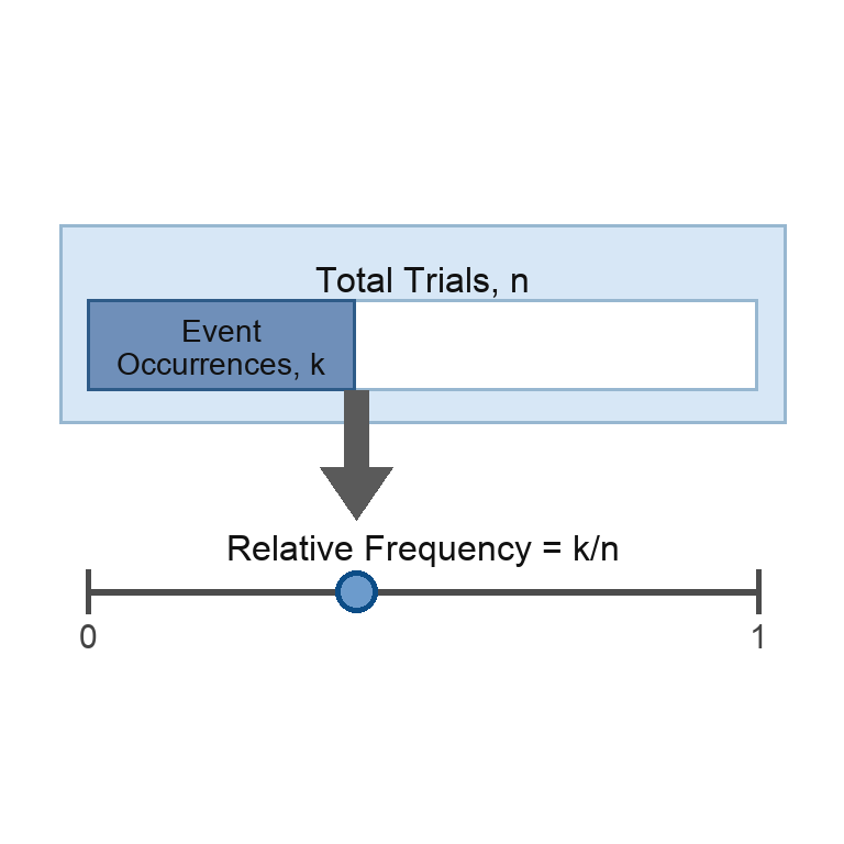
Relative frequency is the proportion of trials in which a specific event occurred. If we conduct an experiment $n$ times in total, and the event we care about occurs $k$ times, then the relative frequency of that event is:

Experiment results can be recorded in many forms, and the method for computing relative frequency stays the same no matter how the data is written down.

For example, results might be organized in a table:

They might be tracked using tally marks:

Or they might simply be written as a list of outcomes:

The calculation always follows the same three-step pattern:

1. Identify the total number of trials, $n$: count how many times the experiment was run, or how many observations were recorded.
2. Count the event occurrences, $k$: go through the data and tally how many times the specific event happened.
3. Divide $k$ by $n$ to obtain the relative frequency.

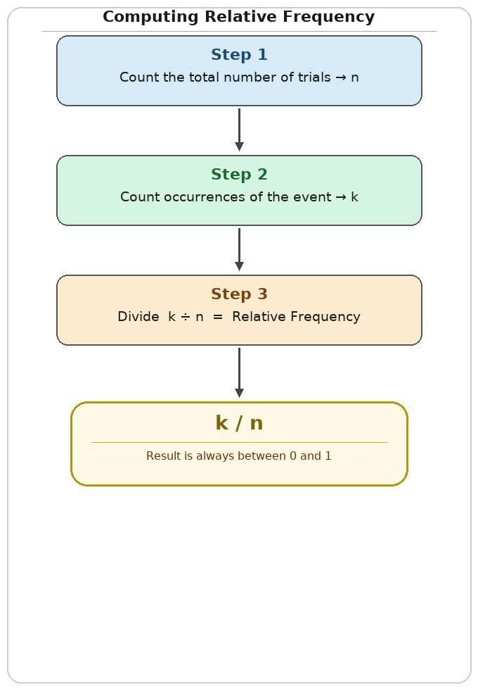
Each step is straightforward on its own. The key is being careful to count only the trials that match the event of interest, and to make sure $$ reflects the number of trials, not just the favorable ones.

Let's see some quick examples using different ways of recording results.

A bag is checked 25 times at an airport, and 4 of those checks find an overweight bag.

So the relative frequency of "overweight bag" is

A store records whether a package arrived damaged.

So the relative frequency of "damaged" is

Suppose a basketball player takes 10 free throws, and the results are recorded as

Suppose we roll a standard six-sided die 30 times and record each result. After all 30 rolls, the outcome "rolling a 3" appeared 7 times.

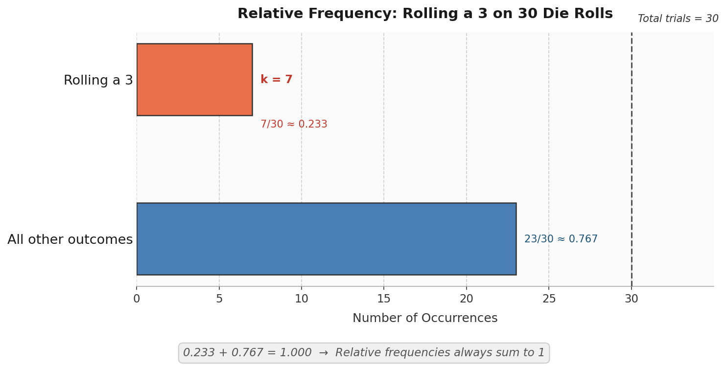
Applying the formula, the relative frequency of rolling a 3 is:

Here is where relative frequency becomes especially meaningful. We do not use it only to describe what happened in the past — we also treat it as our best estimate of the probability that the event will happen in the future. That shift from description to prediction is what makes relative frequency so powerful.

In the die example, our experimental estimate of $P(\text{rolling a 3})$ is approximately $0.233$. If the die were perfectly fair, the theoretical value would be

In this lesson, you learned that relative frequency measures how often an event occurs in proportion to the total number of trials, computed as $\frac{k}{n}$. Like theoretical probability, this value always falls between 0 and 1, and the relative frequencies of all outcomes in an experiment sum to 1. Most importantly, relative frequency is not just a description of past data — it is your best experimental estimate of the probability of a future event.

The practice exercises ahead will give you hands-on experience computing relative frequency across a range of real-world scenarios, from coin flips to bus arrivals to package deliveries. As you work through each one, pay attention to how the same three-step process applies regardless of context. In the next lesson, we will take a closer look at what happens when the number of trials is very small — and why that matters for the reliability of your estimates.