Filtering with Evidence
Introduction
Welcome back to Probability as a Degree of Belief! You are now on lesson three of five, which means we have crossed the halfway mark of this course. So far, you know how to place your confidence on a -to- scale and you understand that a belief-based probability is provisional — always ready to shift when new information comes along.
That raises a practical question: what groundwork do we need before we can revise probabilities responsibly? The answer starts with a deceptively simple idea called conditional probability. By the end of this lesson, you will be able to read, set up, and compute conditional probabilities from two-way tables and real-world scenarios, and you will see exactly why "given that" means narrowing your attention to only the cases where the evidence holds.
Filtering by Evidence
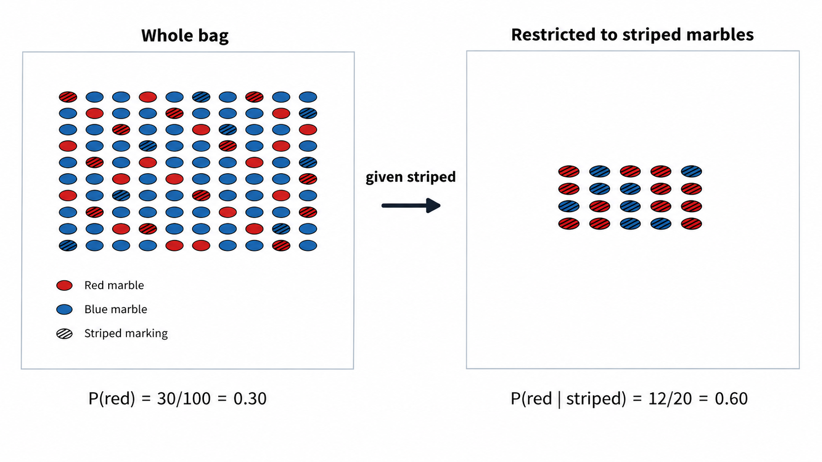
Before we touch any formula, let's build a mental picture. Imagine you have a bag of 100 marbles: 30 are red and 70 are blue. If someone asks, "What is the probability that a randomly chosen marble is red?" the answer is straightforward: .
Now suppose a friend peeks into the bag and tells you, "The marble I picked has a stripe on it." You happen to know that 20 marbles in the bag have stripes, and 12 of those 20 are red. Should you still say the probability of red is ?
Not at all. The evidence has changed your world. Instead of thinking about all 100 marbles, you now restrict your attention to only the 20 striped ones. Among those 20, 12 are red, so your updated probability is . The evidence acted like a filter, shrinking the set of possibilities you care about and producing a new, sharper probability.
This "narrowing of attention" is the heart of conditional probability. Every time you condition on evidence, you are stepping inside a smaller room and counting only what is there.
The Notation: P(Claim | Evidence)
Mathematicians write the probability of a claim given some evidence as:
The vertical bar "" is read as "given that" or simply "given." Everything to the right of the bar is the evidence we accept as true; everything to the left is what we want to know the probability of.
In our marble example, we would write:
Compare this to the unconditional probability , which considers the entire bag. The only thing that changed is the group we are looking at: the denominator shifted from all marbles to just the striped ones. Here is the general recipe:
That denominator is the key. Conditioning on evidence means the evidence becomes your whole world, and you count only within it.
Two-Way Tables as Evidence Maps
When data is organized into a grid, computing conditional probabilities becomes almost automatic. A two-way table (sometimes called a contingency table) cross-classifies a group of cases along two dimensions, letting you read off counts at a glance.
Here is an example. Suppose we survey 200 students about whether they studied for an exam and whether they passed.
| Passed | Did Not Pass | Total | |
|---|---|---|---|
| Studied | 72 | 18 | 90 |
| Did Not Study | 40 | 70 | 110 |
| Total | 112 | 88 | 200 |
Every cell in the interior represents a specific combination. For instance, 72 students both studied and passed. The row and column totals (called marginals) give us the overall count for each single category. Think of the table as a map: once you know which evidence you are conditioning on, you simply walk to the matching row or column, and the rest of the table fades away.
Computing Conditional Probability Step by Step
Let's put that table to work. The question: What is the probability that a student passed, given that they studied?
In notation, we want . Follow these steps:
- Identify the evidence. The evidence is "studied." This tells us which row to restrict our attention to.
- Find the evidence total. The "Studied" row has a total of 90 students. This becomes our denominator.
- Find the overlap. Within those 90 students, 72 also passed. This is our numerator.
- Divide.
Among the students who studied, 80% passed. Notice we completely ignored the 110 students who did not study — they fall outside our evidence filter.
For comparison, the unconditional probability of passing (using all 200 students) is . The evidence "studied" raised the probability from to , because the subset of students who studied has a higher pass rate than the overall group.
Choosing the Right Denominator
The most common mistake with conditional probability is picking the wrong denominator. To see why, let's ask a different question from the same table: What is the probability that a student studied, given that they passed?
Now our evidence is "passed," so we restrict attention to the 112 students who passed. Among those, 72 studied. Therefore:
Notice this is a different number from . The numerator (72) is the same in both cases because it counts the same overlap group. What changed is the denominator — the group we conditioned on.
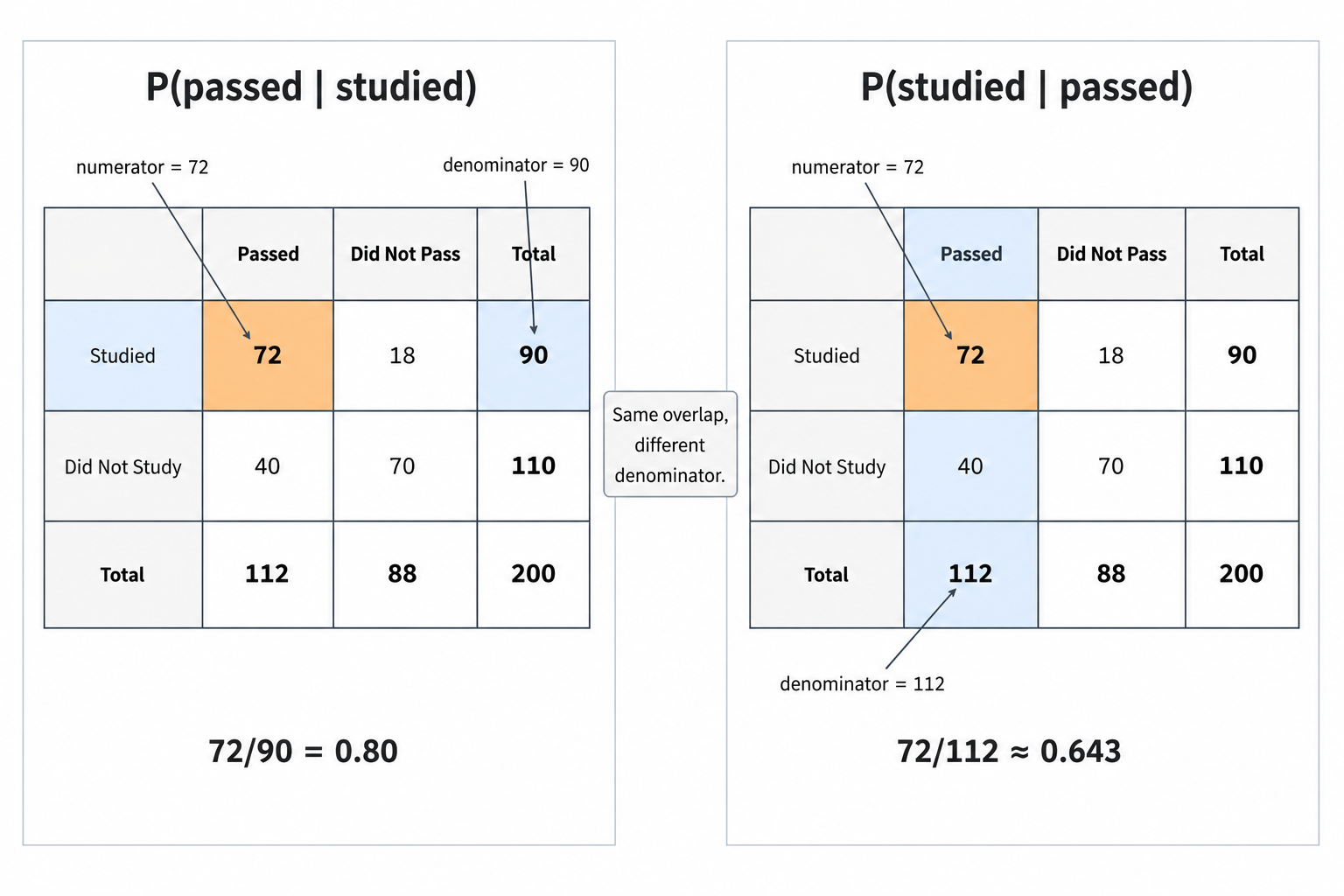
Swapping the two sides of the bar produces a genuinely different probability, and exploring why that matters will be the focus of our very next lesson. For now, keep this quick rule of thumb: the group named after the bar is always the denominator.
Conditional Probability from a Stated Scenario
Not every problem hands you a neat table. Sometimes the data lives in a sentence or a report, and you need to set up the conditional probability yourself. The logic, though, never changes.
Suppose a weather service reports that on 60 out of the last 200 days it rained, and on 45 of those rainy days the temperature was below 15 °C. We want .
The evidence is "rain." Out of 200 days, 60 had rain — that is our restricted world. Of those 60 days, 45 had temperatures below 15 °C. So:
Whether data arrives in a table, a paragraph, or a real-time dashboard, the steps are identical: identify the evidence, find its total, count the overlap, and divide. The mental move is always the same — step inside the evidence group, then look around.
Conclusion and Next Steps
Here are the core ideas to carry forward. Conditional probability, written , works by narrowing your attention to only the cases where the evidence holds and then measuring the claim within that smaller group. In a two-way table, the evidence picks out the row or column that becomes your denominator, and the overlap cell becomes the numerator. This narrowing-of-attention operation is one of the core tools that will later power Bayesian belief updates.
Time to put these ideas into action! In the exercises that follow, you will describe how conditioning filters a real dataset, compute conditional probabilities from two-way tables with different conditioning groups, and explain in your own words why restricting attention to the evidence changes the numbers. Let's dive in!
