Welcome back! In the previous lesson, you learned how to clean and prepare PredictHealth’s customer database, ensuring your data is reliable and ready for modeling. You now understand how to handle missing values, treat outliers, normalize features, and encode categorical variables. With a clean dataset in hand, you are ready to take the next step: building, validating, and evaluating predictive models in a way that ensures they perform well not just on your current data, but also on new, unseen data.

In this lesson, you will learn about PredictHealth’s model validation strategy. You will discover why it is important to split your data into different subsets, how to build a robust modeling pipeline, and how to evaluate your model’s performance using a variety of metrics and visualizations. By the end of this lesson, you will be able to confidently train, validate, and test your models, ensuring they are both accurate and reliable. You will also get a first look at cross-validation, a powerful technique for making the most of your data. Let’s get started!

Before you train a predictive model, it is essential to split your data into separate parts. This is not just a formality — it is a best practice that helps you build models that generalize well to new data. You may remember this idea from earlier lessons, but now we will go deeper and use three distinct subsets: the training set, the validation set, and the test set.

The training set is used to fit the model. The validation set helps you tune the model and check its performance during development, allowing you to make adjustments without biasing your final results. The test set is kept completely separate until the very end, providing an unbiased evaluation of your model’s true performance on unseen data.

In practice, a common split is 70% for training, 15% for validation, and 15% for testing. Here is how you can do this using scikit-learn’s train_test_split function:

The output might look like this:

This approach ensures that each subset serves its purpose, helping you avoid overfitting and giving you a realistic sense of how your model will perform in the real world.

Now that your data is split, it is time to build a pipeline that handles all the necessary preprocessing steps and the model itself. You have already learned about pipelines and one-hot encoding in previous lessons, so this will be a reminder with a few new details.

A pipeline in scikit-learn allows you to chain together preprocessing steps (like encoding categorical variables and passing through numerical features) with your model. This ensures that every time you train or test your model, the data is processed in exactly the same way.

Here is how you can create a pipeline that preprocesses both numerical and categorical features, then fits a linear regression model:

This pipeline first applies the appropriate transformations to your features, then fits the regression model. By using a pipeline, you reduce the risk of data leakage and make your workflow more organized and reproducible.

With your pipeline ready, you can now train your model using the training data. After training, you will evaluate its performance on the validation set. This step helps you understand how well your model is learning and whether it is likely to generalize to new data.

To train the model, simply call the fit method on your pipeline with the training data. Then, use the predict method to generate predictions on the validation set. You can measure performance using several metrics:

• Mean Squared Error (MSE): The average squared difference between actual and predicted values.
• Root Mean Squared Error (RMSE): The square root of MSE, which brings the error back to the original units.
• Mean Absolute Error (MAE): The average absolute difference between actual and predicted values.
• R-squared (R²): The proportion of variance in the target variable explained by the model.

Here is how you can do this in code:

A sample output might be:

These metrics give you a clear sense of how well your model is performing on data it has not seen during training.

Once you are satisfied with your model’s performance on the validation set, it is time for the final test. The test set has been kept separate from all previous steps, so it provides an unbiased estimate of how your model will perform on truly new data.

You use the same approach as before: generate predictions on the test set and calculate the same metrics. This step is crucial for understanding the real-world effectiveness of your model.

Here is the code:

A typical output might look like:

If your test set results are similar to your validation set results, it means your model is generalizing well and is not overfitting.

While splitting your data into training, validation, and test sets is a strong approach, sometimes you want an even more reliable estimate of your model's performance. This is where cross-validation comes in. Cross-validation involves splitting your data into several folds, training and testing the model on different combinations, and averaging the results.

When should you use each approach? If you have abundant data (typically thousands of samples), the three-way split (train/validation/test) is often preferred because it gives you a dedicated test set that remains completely untouched until final evaluation. However, when data is scarce, k-fold cross-validation makes better use of your limited samples by ensuring every data point gets used for both training and validation.

Cross-validation is particularly useful for model selection — comparing different algorithms or tuning hyperparameters — because it gives you a more stable estimate of performance across multiple data splits. However, it comes with a computational cost: you are essentially training your model k times instead of once, which can be significant for complex models or large datasets. For final model evaluation, many practitioners still prefer a held-out test set that has never been used in any training or validation process.

A common method is 5-fold cross-validation, where the data is split into five parts. Each part gets a turn as the validation set, while the others are used for training. This helps you see how your model performs across different subsets of the data.

In scikit-learn, you can use the cross_val_score function to do this easily. Here is an example:

The output might be:

Cross-validation gives you a more robust sense of your model's stability and helps you avoid being misled by a lucky or unlucky split.

Numbers are important, but sometimes a picture is worth a thousand words. Visualizing your model's predictions can help you spot patterns, strengths, and weaknesses that metrics alone might miss.

One useful plot is the actual vs. predicted scatter plot. This shows how close your model's predictions are to the true values. Ideally, the points should fall along a diagonal line.

Here is how you can create this plot:

You will see a scatter plot where each point represents a prediction. The closer the points are to the dashed line, the better your model is performing.

Another helpful visualization is the residual plot, which shows the difference between actual and predicted values (the residuals) against the predicted values. This can help you spot patterns that suggest your model is missing something.

Here is the code:

If the residuals are randomly scattered around zero, it means your model's errors are evenly distributed, which is a good sign.

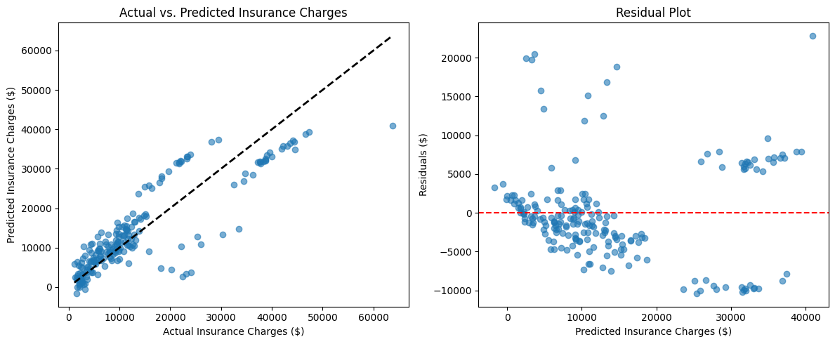
In the residual plot above, you can see a typical example of how residuals should look for a well-performing model. The points are scattered roughly evenly around the horizontal red line (which represents zero error), without showing any clear patterns or trends. This random distribution of residuals indicates that your model's errors are not systematically biased in any particular direction.

Notice that most residuals fall within a reasonable range around zero, though there are a few outliers with larger positive and negative residuals. This is normal and expected. If you saw a clear pattern in the residuals — such as a curve, a funnel shape, or clustering — it would suggest that your model is missing some important relationships in the data that could be captured with additional features or a different modeling approach.

In this lesson, you learned how to validate and evaluate predictive models using a structured approach. You now know why it is important to split your data into training, validation, and test sets, and how each subset helps you build better models. You practiced building a preprocessing and modeling pipeline, training your model, and evaluating its performance using key metrics and visualizations. You also got an introduction to cross-validation, which provides an even more reliable estimate of model performance.

You are now ready to put these concepts into practice. In the next set of exercises, you will apply what you have learned to real data, building and validating your own models in the CodeSignal environment. Remember, careful validation is the key to building models you can trust. Great work getting this far — let’s continue building your skills!