Welcome back to the PredictHealth's Advanced Pricing System course. In the previous lesson, you learned how to model non-linear cost patterns in health insurance data using polynomial regression. You saw how features like age and BMI can have complex, curved effects on insurance charges, and you practiced building models that can capture these patterns. In this lesson, we will take your modeling skills a step further by exploring feature interactions - situations where the effect of one variable depends on the value of another. For example, the impact of being a smoker on insurance costs might be much greater for individuals with high BMI than for those with normal BMI, because health risks compound when smoking is combined with obesity. By the end of this lesson, you will know how to create interaction features, include them in your regression models, evaluate their impact, and visualize their effects to build more accurate and realistic pricing models.

In real-world insurance pricing, it is common for the effect of one factor to depend on another. This is what we call a feature interaction. For example, while both BMI and smoking status individually affect insurance costs, their combined effect can be much larger than the sum of their separate effects. In other words, being a smoker with high BMI may increase costs much more than just being a smoker or just having high BMI.

To make this concrete, imagine two smokers: one has a BMI of 25 (normal weight), and the other has a BMI of 35 (obese). The extra cost for smoking is not the same for both; it is usually much higher for the person with higher BMI. This is because the health risks of smoking compound with obesity-related health issues, and insurance companies need to account for this in their pricing. By including interaction terms in your model, you can capture these kinds of complex relationships and make your predictions more accurate.

To include interaction effects in your model, you first need to create new features that represent these interactions. In the PredictHealth dataset, we have both numeric and categorical variables. For example, the smoker column is categorical, with values "yes" or "no." To use it in mathematical operations, we need to convert it to a numeric format. This is often done by mapping "no" to 0 and "yes" to 1.

Once you have numeric versions of your variables, you can create interaction features by multiplying them together. For example, to capture the interaction between BMI and smoking status, you can create a new feature called bmi_smoker by multiplying the bmi column by the numeric version of smoker. Similarly, you can create age_smoker to capture the interaction between age and smoking status.

Here is how you can do this in code:

After running this code, your dataset will have new columns that represent the combined effects of these features. These interaction terms will help your model learn more about how different factors work together to influence insurance charges.

Now that you have created interaction features, the next step is to include them in your regression model. You will also need to prepare your data by converting any remaining categorical variables, such as sex and region, into dummy variables. This allows the regression model to use all the information in the dataset.

After preparing the data, you can split it into training and testing sets, just as you did in the previous lesson. Then, you can fit a linear regression model that includes both the original features and the new interaction terms.

Here is how you can prepare the data and train the model:

By including the interaction terms in your model, you are giving it the ability to learn more complex relationships in the data. This often leads to better predictions, especially when the real-world effects are not simply additive.

After training your model, it is important to evaluate how well it performs. As a reminder from the previous lesson, two key metrics for regression models are RMSE (Root Mean Squared Error) and R² (R-squared). RMSE tells you how far off your predictions are, on average, while R² shows how much of the variation in the data is explained by your model.

You can also look at the model's coefficients to understand the impact of each feature, including the interaction terms. This helps you interpret the business meaning of your model.

Here is how you can evaluate the model and analyze the coefficients:

A sample output might look like this:

From this output, you can see that the bmi_smoker interaction has a very large positive coefficient (1470.48), meaning that each unit increase in BMI makes smoking much more expensive. This demonstrates how BMI and smoking status interact to compound health insurance costs.

Important Note: While interactions can improve model accuracy, adding too many can lead to overfitting, where the model performs well on training data but poorly on new data. Always validate your model on unseen data and consider using cross-validation to get a more robust performance estimate. Focus on interactions that make business sense rather than adding all possible combinations.

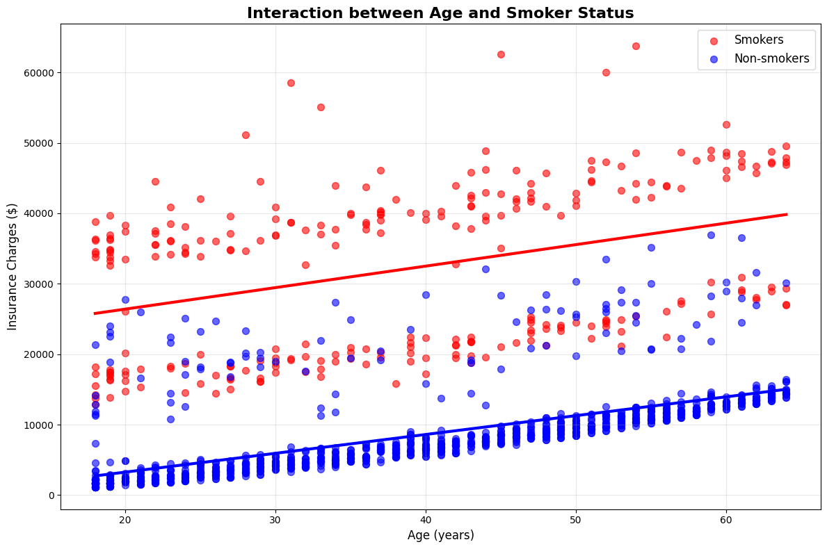
Visualization helps you understand how feature interactions affect your predictions. A common approach is to plot the relationship between a key feature and the target variable, separating the data by another feature. For example, plotting insurance charges against BMI with different colors for smokers and non-smokers shows how the effect of BMI changes depending on smoking status.

Here is how you can create such a plot:

This plot shows two different trends: one for smokers and one for non-smokers. You can notice that the slope for smokers is much steeper, meaning that insurance costs increase much faster with BMI for smokers than for non-smokers, providing visual evidence for the importance of including the BMI-smoking interaction term in your model.

In this lesson, you learned how to identify and model feature interactions in health insurance pricing data. You saw how the effect of one variable, such as BMI, can depend on another variable, like smoking status, and how to create new features to capture these interactions. You practiced including these interaction terms in a regression model, evaluated the model's performance, and interpreted the coefficients to understand their business impact. The key insight is that BMI-smoking interaction is often the strongest predictor in insurance pricing models, as health risks compound when smoking is combined with obesity. Finally, you visualized the interactions to see how they affect insurance charges in real-world data.

You are now ready to apply these concepts in hands-on practice exercises. In the next section, you will have the opportunity to create your own interaction features, build models, and interpret the results. This will help you gain confidence in using feature interactions to improve the accuracy and realism of your pricing models.