Imagine a savings account that earns the same percentage each month. The amount added in the second month may be larger than the amount added in the first month, even though the interest rate has not changed, because each percentage is applied to a new balance. This pattern of repeated multiplication is the central idea behind exponential functions.
You have completed the first two lessons of Nonlinear Graphs and Key Features, and you are now entering the third of six lessons—the midpoint of the course. Earlier, you used vertices and symmetry to construct quadratic and absolute-value graphs; now, you will use an initial value, a multiplication factor, and a value table to build a different type of graph.
By the end of this lesson, you will be able to:
Evaluate simple exponential expressions, including expressions with negative exponents.
Identify exponential growth and decay from the base.
Construct an exponential graph from a value table.
Locate the y-intercept and horizontal asymptote.
Explain how exponential change differs from linear change.
Consider the pattern 1,2,4,8,16. Each value is found by multiplying the previous value by 2. This is different from the linear pattern 1,3,5,7, where each value is found by adding 2.
The rule 2x describes repeated multiplication. For example, 23=2⋅2⋅2=8. When x increases by 1, the output is multiplied by 2; when x decreases by 1, the output is divided by 2.
Negative exponents describe those values to the left of x=0:
2−1=21,2−2=221=41
The negative sign in the exponent does not make the output negative; it tells you to use a reciprocal. This is why the graph of y=2x gets closer to the x-axis as it moves left, while its outputs grow rapidly as it moves right. That repeated-multiplication pattern, rather than a vertex or line of symmetry, will guide the graphing process.
The Basic Exponential Family
A simple exponential function is commonly written as
y=Abx
For this lesson, assume A>0 and b>0. A changing exponential function also requires b=1; when b=1, the function is constant.
Part
Meaning
A
The initial output, or the value when x=0
b
The multiplication factor for every one-unit increase in x
x
The input and exponent
Because b0=1, the output when x=0 is
y=Ab0=A(1)=A
Therefore, the graph has the y-intercept (0,A). The repeated-multiplication rule can also be shown algebraically:
f(x+1)=Abx+1=b(Abx)=bf(x)
So moving one unit to the right multiplies the previous output by b.
For positive A, every output is positive. In the direction where the outputs become very small, the graph approaches the line y=0; this line is called the horizontal asymptote. For a basic exponential function, the y-intercept and horizontal asymptote take the place of the vertex and symmetry line used in the previous lesson.
Join the 1M+ learners on CodeSignal
Be a part of our community of 1M+ users who develop and demonstrate their skills on CodeSignal
The base tells you whether the graph rises or falls as x increases. Compare the base with 1, not simply with 0.
Base condition
Behavior as x increases
Relative change per step
Example
b>1
Exponential growth
Increase by b−1
2x
0<b<1
Exponential decay
Decrease by 1−b
(21)x
b=1
Constant output
No change
1x=1
For example, a base of 1.08 means that each output is multiplied by $1.08, or increased by 8%. A base of 0.92 means that each output is multiplied by $0.92, or decreased by 8%.
The base also determines the direction of the horizontal asymptote. For b>1, outputs approach 0 as x becomes very negative. For 0<b<1, outputs approach 0 as x becomes very large. With this classification in place, you are ready to construct a growth graph.
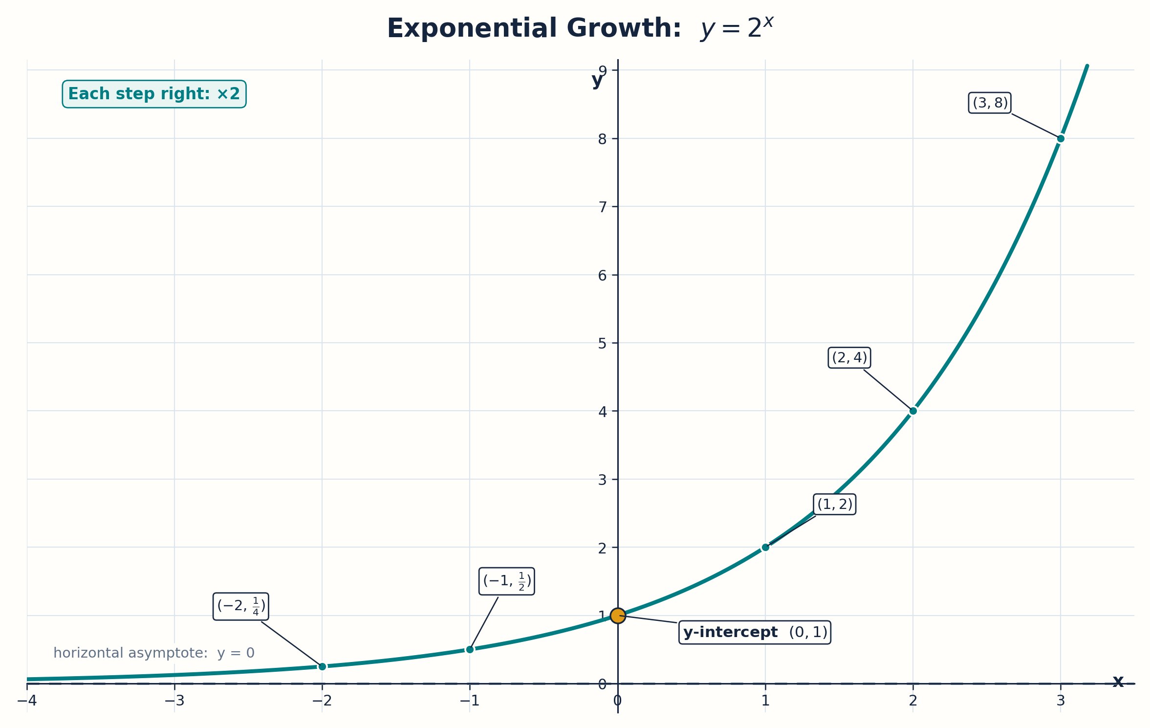
Consider the basic exponential growth function
y=2x
Use several inputs on both sides of x=0 so the table shows the graph’s behavior:
x
−2
−1
0
1
2
3
y=2x
41
21
1
2
4
8
The table gives the points
(−2,41),(−1,21),(0,1),(1,2),(2,4),(3,8)
Plot the points and connect them with one smooth curve. The curve rises slowly on the left and becomes steeper as x increases.
Important features of this graph include:
It is increasing because the base 2 is greater than 1.
Its y-intercept is (0,1) because 20=1.
Its horizontal asymptote is y=0, approached as x→−∞.
Its domain is all real numbers, and its range is y>0.
It never crosses or touches y=0 because 2x is positive for every real x.
The next example uses a base between 0 and 1. The multiplication factor will then make the graph decrease as it moves to the right.
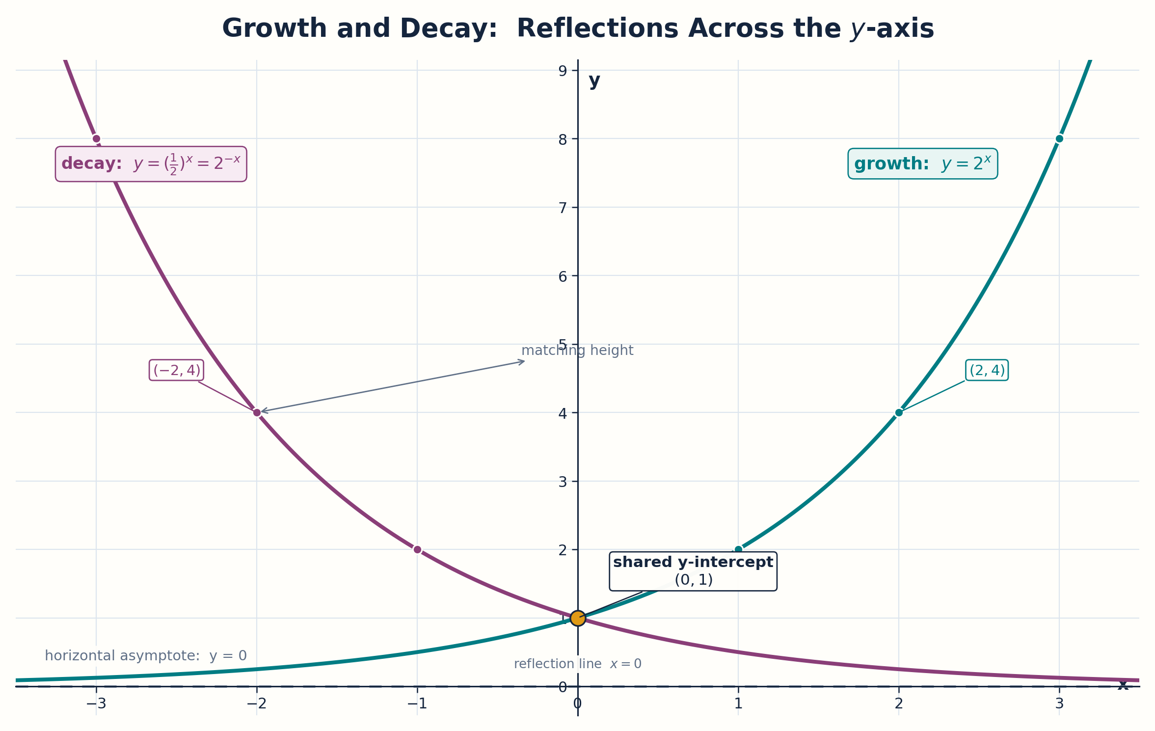
Now consider
y=(21)x
The base is between 0 and 1, so the function represents exponential decay:
x
−2
−1
0
1
2
3
y=(21)x
4
2
1
21
41
81
Each time x increases by 1, the output is multiplied by 21. In other words, the output is cut in half at every step. Also,
(21)x=2−x
so this decay graph is the growth graph y=2x reflected across the y-axis.
Feature
Result for y=(21)x
Direction
Decreasing as x increases
y-intercept
(0,1)
Horizontal asymptote
y=0, approached as x→∞
Domain
All real numbers
Range
y>0
At the far left, the outputs become large; at the far right, they get closer to 0. The base controls the direction of change, while the coefficient A controls the initial output.
Return to the general form
y=Abx
The coefficient A sets the output at x=0 and scales every output by the same amount. Consider
y=3⋅2x
The base is still 2, so the function doubles each time x increases by 1. However, it starts at 3 instead of 1.
x
−1
0
1
2
3
y=3⋅2x
1.5
3
6
12
24
The y-intercept is (0,3). Compared with y=2x, every output is multiplied by 3, so the graph is vertically scaled while keeping the same growth factor and horizontal asymptote.
The same idea works for decay. The function
y=4(21)x
starts at 4 and halves as x increases. Its y-intercept is (0,4), and its horizontal asymptote remains y=0. This lesson focuses on A>0; a negative value of A would reflect the graph across the x-axis.
A linear function changes by a constant amount, while an exponential function changes by a constant factor. This difference appears in both the value table and the graph.
Feature
Linear function
Exponential function
Common form
y=mx+c
y=Abx
Change between outputs
Constant difference
Constant ratio
Graph shape
Straight line
Smooth curve
Rate of change
Constant slope
Changing slope
For the same inputs x=0,1,2,3, the linear function y=2x+1 produces 1,3,5,7. The differences are always +2. The exponential function y=2x produces 1,2,4,8; the differences change, but each output is twice the previous one.
This explains why exponential growth can look almost flat at first and then become steep. A straight line keeps the same slope, but an exponential growth graph continually changes its slope as its outputs get larger.
Exponential functions are useful when a quantity changes by the same percentage or factor during each time period. For example,
P(t)=500(1.08)t
could model a population that begins at 500 and grows by 8% each year. The initial value is P(0)=500, and the base 1.08 means that each year’s population is 1.08 times the previous year’s population.
A decay model might be
V(t)=1200(0.85)t
This could represent an item that begins with a value of 1200 and keeps 85% of its value each year. The decrease is 15% of the current value, not a fixed decrease of 15 units. In a real model, t might be restricted to t≥0 because negative years may not make sense, even though the equation itself accepts any real input.
For a function in the simple form y=Abx, use the following routine:
Identify A and b. Treat A as the initial value and b as the repeated multiplication factor.
Classify the behavior. If b>1, expect growth; if 0<b<1, expect decay.
Find the y-intercept. Substitute x=0 to get the point (0,A).
Choose several inputs. Include negative, zero, and positive values when possible.
Complete the value table. For negative exponents, use reciprocals; moving one step to the right multiplies the previous output by b.
Plot the points on a coordinate plane.
Draw a smooth curve through the points and mark the horizontal asymptote y=0.
Check the graph. Growth should rise to the right, decay should fall to the right, and the graph should pass through (0,A).
A few carefully chosen points are usually enough to show the pattern. The goal is not to calculate every output, but to represent the graph’s direction, steepness, intercept, and end behavior accurately.
Use these checks when you evaluate or sketch an exponential function:
Calling every positive base growth: A base such as 0.4 produces decay because it is less than 1.
Adding instead of multiplying: In y=3⋅2x, each step multiplies the previous output by 2; it does not add 2.
Confusing A and b:A gives the output at x=0, while b controls the repeated factor.
Forgetting exponent rules: Remember that b0=1 and b−n=bn1.
Using the percentage as the base: An 8% increase uses the base 1.08, not 0.08.
Drawing through the asymptote: For positive A, the graph approaches y=0 but does not reach or cross it.
Using straight line segments: Exponential graphs should be drawn as smooth curves, not as a collection of connected line segments.
A simple exponential function has the form y=Abx.
A is the initial output and gives the y-intercept (0,A).
b is the multiplication factor for each one-unit increase in x.
If b>1, the graph shows growth; if 0<b<1, it shows decay.
Exponential tables have constant ratios, while linear tables have constant differences.
For positive A, the graph has domain all real numbers, range y>0, and horizontal asymptote y=0.
A value table provides the points needed to draw the smooth exponential curve.
You can now read a simple exponential equation as a graphing plan: A gives the starting value, b gives the repeated factor, and a value table supplies points. Growth and decay have different end behavior, but both can be sketched with a smooth curve and a horizontal asymptote.
In the practice section, you will evaluate expressions with positive and negative exponents, complete value tables, and sketch growth and decay graphs. You will also use intercepts, ratios, and asymptotes to check whether a graph matches its equation.