Quartiles and IQR

Welcome back to Measuring Spread with Range and IQR! You are now on the second of five lessons in this course, and you have already built a solid foundation. In the previous lesson, we computed the range and saw its biggest weakness: because it depends on only the maximum and minimum, a single extreme value can inflate it dramatically. That raises an important question: is there a way to measure spread that is far less sensitive to the extremes? The answer is yes, and it is what this lesson is all about. Here we introduce quartiles and the interquartile range (IQR), two tools that focus on the middle of the data and let values at the edges fade into the background.

Think of the range as measuring a room from wall to wall. That gives you the total width, but it reveals nothing about where the furniture sits. To understand how values are actually arranged, we need landmarks inside the dataset, not just at its edges.

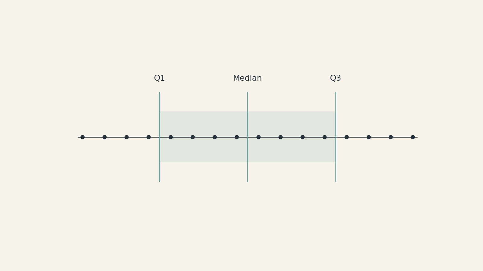
Quartiles give us exactly those landmarks. They divide a sorted dataset into four equal parts, marking the boundaries at the 25%, 50%, and 75% points. By measuring the distance between the 25% and 75% marks, we capture the spread of the central bulk of the data while letting extreme highs and lows stay out of the picture.

Once a dataset is sorted from smallest to largest, three values split it into four quarters:

• Q1 (the first quartile) sits at the 25% mark. About one-quarter of the data falls below this value.
• Q2 (the second quartile) is the median, the 50% mark. As you may recall from the previous course, the median divides the data in half.
• Q3 (the third quartile) sits at the 75% mark. About three-quarters of the data falls below this value.

Here is the core idea: Q1 is the median of the lower half of the data, and Q3 is the median of the upper half. The specific approach we use in this course is called the median-exclusive method. When the dataset has an odd number of values, we set the overall median aside before finding Q1 and Q3 — it does not belong to either half. The next section walks through the full procedure.

Follow these steps every time you need to find quartiles:

1. Sort the data from smallest to largest.
2. Find the median (Q2). If the count is odd, the median is the single middle value. If the count is even, the median is the average of the two middle values.
3. Form the lower half. Take every value that falls below the median position. If the count is odd, do not include the median itself.
4. Form the upper half. Take every value that falls above the median position. Again, exclude the median if the count is odd.
5. Find Q1 as the median of the lower half.
6. Find Q3 as the median of the upper half.

The critical detail is in steps 3 and 4: when the count is odd, the median sits alone in the center and does not belong to either half. That is what makes the method median-exclusive. When the count is even, no value needs to be excluded, and the data splits cleanly into two equal halves.

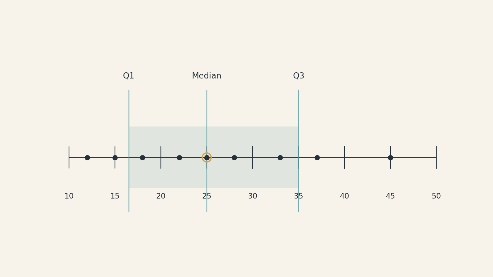
Suppose we recorded daily commute times (in minutes) for nine trips:

The data is already sorted and contains $9$ values. Let's walk through each step.

Find the median. The middle position is position 5, so the median is $25$.

Split the data. We set $25$ aside. The lower half is the four values to its left: $12, 15, 18, 22$. The upper half is the four values to its right: $28, 33, 37, 45$.

Find Q1. The lower half has four values, so Q1 is the average of the two middle ones:

Find Q3. The upper half also has four values:

Our quartiles are $Q1 = 16.5$, $Q2 = 25$, and $Q3 = 35$. The nine trips are now divided into four groups of roughly equal size, with the quartile values serving as boundaries.

Now consider quiz scores for eight students, already in order:

With an even count there is no single middle value to set aside, so the split happens naturally.

Median: The two middle values are $78$ and $84$, giving $Q2 = \frac{78 + 84}{2} = 81$.

The lower half is the first four values: $62, 70, 75, 78$. The upper half is the last four: $84, 88, 91, 96$. Every data point belongs to exactly one half.

When the count is even, you do not need to exclude anything. The two halves form on their own, and you simply find the median of each.

With Q1 and Q3 in hand, the interquartile range is one subtraction away:

For our commute-time example:

For the quiz-score example:

The IQR tells you the width of the interval that contains the middle 50% of the data. In the commute example, the central half of all trips lasted between $16.5$ and $35$ minutes — a span of $18.5$ minutes. That single number summarizes how tightly or loosely the typical values cluster, without being pulled by the shortest or longest trip in the dataset.

In the previous lesson we saw how one extreme value can inflate the range. The IQR sidesteps most of this problem because it is built from Q1 and Q3, which sit safely inside the data.

Return to our commute data: $12, 15, 18, 22, 25, 28, 33, 37, 45$. Now imagine one trip hit unusual traffic and took $120$ minutes instead of $45$:

The range more than triples, jumping from $33$ to $108$. The IQR does not budge in this case. Replacing the largest value with a much bigger one leaves Q1 and Q3 unchanged because those quartiles are computed from the middle portion of the dataset rather than the extremes.

This resistance to outliers makes the IQR a more stable and reliable measure when your goal is to describe how spread out the typical values are. The range still has its place as a quick first look, but the IQR is the better tool whenever extreme observations are present or possible.

It is worth being precise here: the IQR is highly resistant to outliers but not perfectly immune to them. In smaller datasets especially, adding or removing an extreme value changes the dataset's size, which can shift the positions of Q1 and Q3 and slightly change the IQR. The key takeaway is that the IQR is far more stable than the range in the presence of extremes — not that it is unaffected by them.

In this lesson you learned how to split a sorted dataset into four quarters using Q1, the median (Q2), and Q3 via the median-exclusive method. The interquartile range, $\text{IQR} = Q3 - Q1$, captures the spread of the middle 50% of the data and stays steady even when extreme values would send the range soaring.

Up next, we will combine the quartiles with the minimum and maximum to build the five-number summary, a compact snapshot of an entire distribution. But first, jump into the practice exercises to find quartiles in both odd and even datasets, compute the IQR, and see for yourself just how much steadier the IQR can be when outliers try to steal the show!