Outliers Mean and Median
Welcome to Lesson Four
Welcome back to Measures of Center! We are on lesson four of five, so we are nearly at the finish line. Over the previous three lessons, we built up three ways to summarize the center of a dataset: the mode (most frequent value), the median (middle value), and the mean (sum divided by count). Today we put two of those measures to the test by asking a simple but important question: what happens when one value in the dataset is far away from the rest?
By the end of this lesson, we will see clearly that the mean is sensitive to extreme values while the median is resistant, and we will understand the reasons behind each response.
What Is an Outlier?
Before we explore the effects, let's make sure we share a common vocabulary. An outlier is a data value that is much larger or much smaller than the rest of the values in a dataset. Think of a quiet residential street where most homes sell for around $250,000, but one sprawling estate is listed at $1.2 million. That estate's price would be an outlier.
Outliers can appear for many reasons: a data-entry error, an unusual circumstance, or simply natural variation. Regardless of why they show up, they can change the story our summary statistics tell. The key question for this lesson is: which measure of center do they affect more, and why?
A Small Office Before the Outlier
Imagine five employees at a small marketing firm. Their annual salaries, in thousands of dollars, are:
Let's compute both the median and the mean using the skills we practiced in the last two lessons.
Median: The data are already sorted, and the middle value (the 3rd of 5) is . So the median salary is $40,000.
Mean:
The mean salary is also $40,000. Both measures agree perfectly, and $40,000 feels like a fair description of a "typical" salary at this firm. Let's see what happens when we disrupt that agreement.
Adding an Extreme Value
Now the firm brings on a new executive whose salary is $150,000. Our dataset becomes:
Let's recalculate both measures with this addition.
Median: With six values, the median is the average of the 3rd and 4th values: . The new median is $41,000.
Mean:
The new mean is about $58,333. Here is the before-and-after comparison:
| Measure | Without Executive | With Executive | Change |
|---|---|---|---|
| Median | $40,000 | $41,000 | +$1,000 |
| Mean | $40,000 | $58,333 | +$18,333 |
A quick dot plot makes the different shifts easier to see:
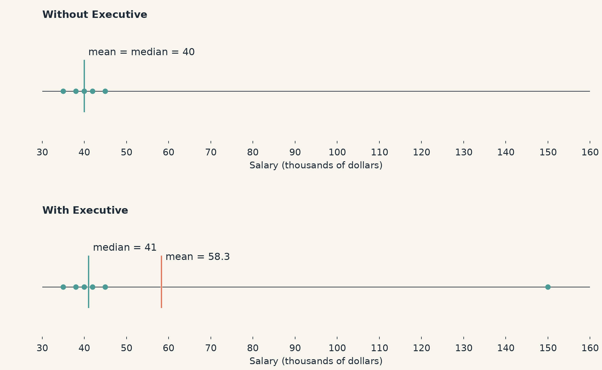
The median shifted by just $1,000, while the mean jumped by over $18,000. Notice that the new mean of $58,333 is higher than the salary of every original employee. It no longer reflects what a "typical" worker at the firm earns. That dramatic gap between the two measures is a direct consequence of how each one is built.
Why the Mean Moves So Much
Recall from the previous lesson that the mean is computed by adding every value and dividing by the count. When we drop a value of into a group that was averaging , that large number inflates the total significantly. One extreme value can pull the mean toward it, much like a heavy weight placed at one end of a seesaw drags the balance point in its direction.
Here is a useful way to think about it: the mean "listens" to every value equally, so a single extreme voice can shift the entire conversation. The bigger the gap between the outlier and the rest of the data, the larger the shift.
Why the Median Barely Budges
The median works on a completely different principle. It cares about position, not magnitude. When we sort the data and locate the middle value, it does not matter whether the largest number is , , or — the middle position stays the same.
In our salary example, going from five values to six shifted the median from the 3rd value to the average of the 3rd and 4th values. That small change happened only because the count of data points changed, not because of the size of the new salary. If the executive had earned $60,000 or $600,000, the median would still be $41,000. This positional logic is exactly what makes the median resistant to outliers.
Sensitive vs. Resistant
Statisticians use two handy labels to describe how measures of center respond to extreme values:
- Sensitive (non-resistant): The measure changes noticeably when an outlier is added or removed. The mean is sensitive because every data value feeds directly into the sum.
- Resistant: The measure changes little or not at all in the presence of an outlier. The median is resistant because it depends only on the middle position in the sorted list.
These labels are not judgments — neither means one measure is always better than the other. In fact, the mean's sensitivity can be a strength when we want our summary to reflect the full total, such as when budgeting for expenses. The median's resistance is a strength when we want to describe what is typical in data that contains extremes, like home prices in a neighborhood with one mansion. Understanding how each measure reacts to outliers is the first step toward choosing the right one, which is exactly what we will tackle next.
Conclusion and Next Steps
Today we saw firsthand that adding a single extreme value can drag the mean far from the center of the data while leaving the median nearly unchanged. The reason traces back to how each measure is built: the mean uses every value in its sum, so one unusually large or small number pulls it off course, while the median looks only at the middle position and ignores how far away the extremes sit.
In the next and final lesson of this course, we will bring everything together and learn how to choose the best measure of center — mean, median, or mode — for a given situation. But first, it is time to put today's ideas into practice. The exercises ahead will have us computing means and medians before and after an outlier appears, deciding which measure better represents a "typical" value, and writing our own plain-language explanations of why extreme values behave the way they do.
