Welcome back to our journey through Linear Landscapes of Dimensionality Reduction. Today's lesson focuses on applying Linear Discriminant Analysis (LDA) using R and then diving into feature extraction and selection. Primarily, we'll be utilizing the lda() function from the MASS package. Ready to take the plunge?

Before diving in, let's do a quick revision of LDA, how it works, and its implementation. As we transition to using R today, our first step is to load the dataset we will be working with. We'll use the built-in iris dataset in R:

Here, iris is a data frame containing both the features (sepal and petal measurements) and the target variable (Species).

Our next step is to preprocess our data. We scale the features to have zero mean and unit variance, which is important for optimal LDA performance. In R, we can use the scale() function:

This code standardizes each feature column by subtracting the mean and dividing by the standard deviation.

To properly evaluate our model, we need to ensure that both the training and testing sets contain a representative mix of all classes. The iris dataset is ordered by species, so simply splitting by row number would result in the test set containing only one species, which is not suitable for model evaluation.

Instead, we'll use random sampling to split the data, ensuring that all classes are represented in both sets. We'll use the sample() function to randomly select 80% of the data for training and the remaining 20% for testing:

This approach ensures that both the training and test sets contain a mix of all three species. The print statements show the dimensions and class distributions of the splits, confirming a balanced split.

Let's apply LDA to our data using the lda() function from the MASS package:

We fit the LDA model to our training data and transform it into a lower-dimensional space.

To better understand our LDA model's results, let's visualize the transformed data using ggplot2:

Output: 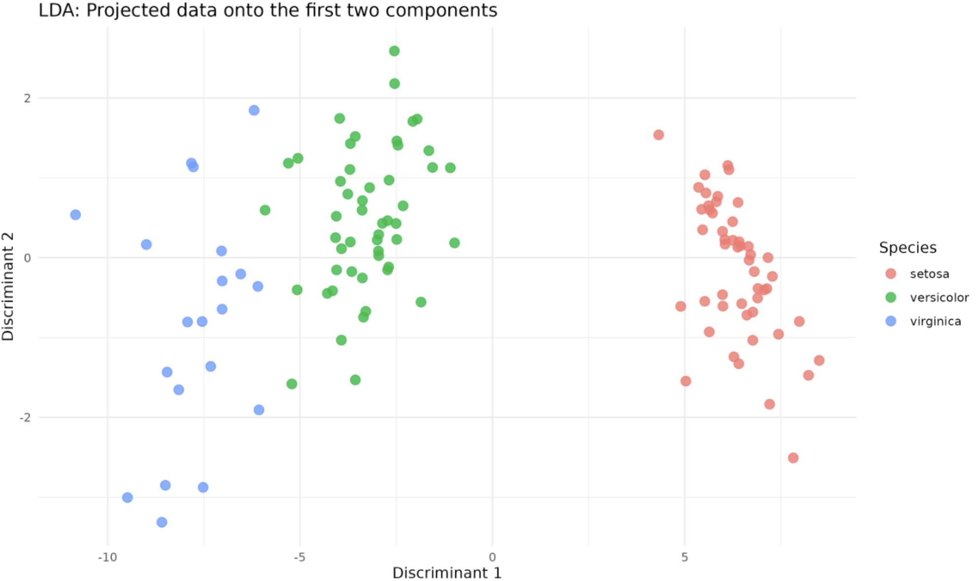This visualization showcases class separation by LDA, easily distinguished by color coding. The Discriminant 1 and Discriminant 2 axes represent the two components we selected for our LDA model — the transformed data is projected onto these axes.

Additionally, LDA can be used as a classifier when the classes are well separated and the assumptions of LDA are met. It's particularly useful for multiclass classification problems.

The predict() function in R can be used to classify new samples. Let's see how to use it:

Here, we use the predict() function from our trained LDA model to predict the classes for our test data and measure its accuracy by comparing the predictions with the actual classes.

We applied LDA using R, performed data extraction and selection, visualized LDA results, and calculated the accuracy of our model. In the next lesson, we'll dive into some hands-on exercises. Remember, practice is pivotal to mastering new concepts and reinforcing learning!