Welcome to the world of Linear Discriminant Analysis (LDA), a technique widely used for dimensionality reduction in supervised learning. In this lesson, we'll explore the concepts behind LDA and build an implementation from scratch using R. For our practical example, we'll use the classic Iris dataset, a well-known dataset in R, to demonstrate how LDA works in practice.

LDA reduces dimensionality by constructing a feature space that optimally separates the classes in the data. The axes in this space are linear combinations of the original features and are known as eigenvectors. The LDA algorithm consists of several steps, such as calculating class mean vectors and scatter matrices, then finding eigenvalues and eigenvectors that map the original feature space onto a lower-dimensional space.

To understand LDA, let's start with a simple two-dimensional example. Suppose we have data points scattered across a 2-D space, with each point belonging to one of two possible classes.

In LDA, we want to project these points onto a line such that, when the points are projected, the two classes are as separated as possible. The goal here is twofold:

1. Maximize the distance between the means of the two classes.
2. Minimize the variation (in other words, the scatter) within each category.

This forms the intuition behind LDA. The crux of an LDA transformation involves formulating a weight matrix and transforming our input data by multiplying it with this weight matrix. The weights here help increase class separability. Let's see how we can achieve this mathematically using scatter matrices.

Let's load the Iris dataset for LDA, which is a 3-class dataset with 4 features. In this example, we'll rename the features to weight_lbs, weight_kgs, and height for demonstration purposes.

# Load required libraries
library(ggplot2)
library(dplyr)

# Load the iris dataset
data(iris)

# Rename features for demonstration
colnames(iris)[1:3] <- c("weight_lbs", "weight_kgs", "height")

# Extract features and target
X <- as.matrix(iris[, c("weight_lbs", "weight_kgs", "height", "Petal.Width")])
y <- as.numeric(iris$Species)

Before proceeding, it's important to consider whether to scale your data for LDA. LDA makes the assumption that each class shares the same covariance structure, and the method is sensitive to the scale of the input features. If your features are measured in different units or have very different variances, those with larger scales can dominate the computation of scatter matrices and the resulting discriminant directions. This can lead to misleading results, as LDA may focus on the features with the largest variances rather than those that best separate the classes.

When to scale:

• If your features are on very different scales (e.g., height in centimeters and weight in kilograms), scaling is recommended.
• If all features are already on a similar scale, scaling may not be necessary.

How to scale:
A common approach is to standardize each feature to have zero mean and unit variance. This ensures that each feature contributes equally to the analysis, and the LDA solution is not biased toward features with larger variances.

Let's standardize the features in our example:

# Normalize the data to zero mean and unit variance
X <- scale(X)

By scaling the data, we help ensure that LDA's assumptions are more closely met and that the resulting discriminant axes are not unduly influenced by the scale of any particular feature.

In R, instead of classes, we typically use lists and functions to encapsulate model state and behavior. We'll define a list to hold the transformation matrix and functions to perform the LDA steps.

LDA <- list()
LDA$W <- NULL

Here, LDA is a list that will store the transformation matrix W after fitting the model.

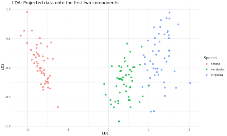
Next, we fit the LDA model, transform the data, and plot the projected samples using ggplot2. We'll use the first two components for visualization.

# Fit LDA and transform data
n_components <- 2
W <- fit_lda(X, y, n_components)
X_lda <- transform_lda(X, W)

# Prepare data for plotting
lda_df <- data.frame(
  LD1 = X_lda[, 1],
  LD2 = X_lda[, 2],
  Species = iris$Species
)

# Plot the transformed data
ggplot(lda_df, aes(x = LD1, y = LD2, color = Species)) +
  geom_point(size = 2, alpha = 0.7) +
  labs(
    title = "LDA: Projected data onto the first two components",
    x = "LD1",
    y = "LD2"
  ) +
    theme_minimal() + theme( panel.background = element_rect(fill = "white", color = NA), plot.background = element_rect(fill = "white", color = NA) )

The output will look like this:

This code creates a scatter plot of the data projected onto the first two linear discriminants, colored by species.

Great job! You've successfully understood the concepts of LDA and its mathematical foundation, and built a simple LDA from scratch using R. Now, get ready for practice exercises to apply your newly acquired knowledge and consolidate your learning! Happy learning!